Akademie věd České republiky. Disertace k získání vědeckého titulu "doktor věd" ve skupině věd fyzikálně-matematických

Transkript

1 Akademie věd České republiky Disertace k získání vědeckého titulu "doktor věd" ve skupině věd fyzikálně-matematických Mathematical analysis of the motion of viscous fluids: motion of incompressible fluid around rotating and translating rigid body, motion of compressible gas, motion of linear viscous fluid in the half space Komise pro obhajoby doktorských disertací v oboru Matematická analýza a příbuzné obory Jméno uchazeče RNDr. Šárka Nečasová, CSc. Pracoviště uchazeče Matematický ústav AV ČR, v. v. i. Místo a datum Praha

2 Contents 1 The motion of viscous fluids around a purely rotating body L q setting Strong solution Weak solution L 2 setting Asymptotic behavior of the motion of viscous fluid around a translating and rotating body Notations, definitions and auxiliary results Main theorems Asymptotic behavior of the viscous fluids in the presence of Coriolis forces Stokes problem in the whole space R Stokes problem in an exterior domain Oseen problem in the whole space R Oseen problem in an exterior domain Compressible motion Free boundary problem for the equation of one-dimensional motion of compressible gas with density-dependent viscosity isentropic case Free boundary problem for the equation of spherically symmetric motion of viscous gas Global existence of solutions for the one-dimensional motions of a compressible viscous gas with radiation: an infrarelativistic model Laplace equation and Stokes problem in the half space Notations Laplace equation Stokes system Generalized solutions to the Stokes system in R N Strong solutions and regularity for the Stokes system in R N Very weak solutions for the Stokes system Stokes problem with Navier condition Weak solutions Strong solutions Very weak solutions List of publications of the dissertation 32 7 Articles included in the dissertation 39 1

3 1 The motion of viscous fluids around a purely rotating body In the first part of the thesis we shall study the time-periodic Oseen equations past a purely rotating body in the whole space and in an exterior domain. Let Ωt) R n n = 2, 3) be given, the time-dependent exterior domain past a rotating body D. We consider that Ω is sufficiently smooth. We assume that Ωt) is filled with a viscous incompressible fluid modelled by the Navier-Stokes equations with the velocity v at infinity. Given the coefficient of viscosity ν > and an external force f = fy, t), we are looking for the velocity ṽ := ṽy, t) and the pressure q := qy, t) solving the nonlinear system ṽ t ν ṽ + ṽ )ṽ + q = f in Ωt), t >, div ṽ = in Ωt), t >, ṽy, t) = ω y on Ωt), t >, ṽy, t) v as y. 1.1) Here denotes the exterior wegde product of R 3, and in the two-dimensional case, ω y = y 2, y 1 ) for y = y 1, y 2 ). Due to the rotation of the body with the angular velocity ω, we have Ωt) = O ω t)ω, where D R n is a fixed exterior domain and O ω t) denotes the orthogonal matrix cos ω t sin ω t ) O ω t) = sin ω t cos ω t cos ω t sin ω t or = if n = ) sin ω t cos ω t 1 After the change of variables x := O ω t) T y and passing to the new functions ux, t) := O T ω ṽy, t) v and px, t) := qy, t), as well as to the force term fx, t) := O ω t) T fy, t), we arrive at the modified Navier Stokes system u t ν u + u )u ω x) )u+ +O ω t) T v )u + ω u + p = f in Ω, t >, div u = in Ω, t >, ux, t) + O ω t) T v = ω x on Ω, t >, ux, t) as x. 1.3) Note that, because of the new coordinate system attached to the rotating body, equation 1.3) 1 contains three new terms, the classical Coriolis force term ω u up to a multiplicative constant) and the terms ω x) )u and O ω t) T v )u which are not subordinate to the Laplacian in unbounded domains. An important step concerns its linearized and steady versions, i.e. either in the whole space R n the modified Stokes systems, 2

4 ν u ω x) )u + ω u + p = f in R n, div u = or g in R n, where n = 2 or n = 3; or in an open set Ω the modified Oseen systems, u as x, 1.4) ν u + k 3 u ω x) )u + ω u + p = f in Ω, div u = or g in Ω, u., t) + u = ω x on Ω, u as x, 1.5) with an appropriate choice of the constant translational velocity at infinity u = ke 3, therefore parallel to ω. We follow two different ways to handle this problem. The first approach in an L 2 - setting uses variational calculus. This viewpoint has already been applied in [23] by R. Farwig and in [58, 59] by S. Kračmar and P. Penel to solve the scalar model equations ν u + k 3 u = f in Ω and with a given non-constant and, in general, non-solenoidal vector function a ν u + k 3 u a u = f in Ω, respectively, in an exterior domain Ω, together with the boundary conditions u = on Ω and u as x. Second, to consider more general weights in L q -spaces, we apply weighted multiplier and Littlewood-Paley theory as well as the theory of one-sided Muckenhoupt weights corresponding to one-sided maximal functions. This approach was firstly introduced by Farwig, Hishida, Müller [27] for the case u = and in [24], [25] when u without weights and then extended to the weighed case by Krbec, Farwig, Nečasová [31], [3] and Nečasová, Schumacher [68]. 1.1 L q setting Definition 1. Let A q, 1 < q <, the set of Muckenhoupt weights, be given by all strictly positive functions w L 1 loc Rn ), for which A q w) := sup Q 1 wq) ) Q 1 w Q) ) q 1 <. 1.6) Q where w := w 1 q 1 and the supremum is taken over all cubes Q in R n. We have excluded the case where w vanishes almost everywhere. For q 1, ), w A q, k 1 N, and an open set Ω, we define 3

5 the Lebesgue space L q wω) := { f L 1 loc Ω) s.t. Ω f q w dx < }, with the norm f q,w := Ω f q w dx ) 1 q, the Sobolev space Hw k,q Ω) := {f L 1 loc Ω) s.t. j f L q wω), j k}, equipped with the norm u k,q,w := k j= j u q,w, the homogeneous Sobolev space Ĥk,q w Ω) := {f L 1 loc Ω) s.t. k f L q wω)}, the space of smooth and compactly supported functions C Ω) and its divergence free counterpart C,σΩ) := {φ C Ω) s.t. div φ = }, and the spaces Ĥk,q w,ω) := C Ω) H b k,q w, H k,q w,ω) := C Ω) Hw k,q. It is easily seen that L q wω)) = L q w Ω) with 1 q + 1 q = 1 and w = w 1 q ) Moreover, by [74], for 1 < q < and w A q there exists s such that 1 s < q and w A s. In addition, if Ω is a bounded domain, then it follows from Hölder s inequality that the weighted Lebesgue spaces are embedded into unweighted ones as follows L q wω) L r Ω) for every r < q/s. 1.8) Considering the dual spaces in 1.8) one obtains that for q and w as above there exists r 1, ) such that L r Ω) L q wω) Strong solution Oseen system see [3] The Oseen system 1.5) has been analyzed by Farwig in [24], [25], in L q -spaces, 1 < q <, the a priori estimates being generalized by Farwig, Krbec, and Nečasová in weighted L q -spaces ν 2 u q,w + p q,w c f q,w, 1.9) More precisely, k 3 u q,w + ω x) u ω u q,w ck, ν, ω) f q,w. 1.1) Theorem 1. Let the weight function w L 1 loc R3 ) be independent of the angular variable θ and satisfy the following condition depending on q 1, ): 2 q < : w τ Ã τq/2 for some τ [1, ) 1 < q < 2 : w τ Ã τq/2 for some τ 2, ] 1.11) 2 q 2 q. 4

6 i) Given f L q wr 3 ) 3 there exists a solution u, p) L 1 loc R3 ) 3 L 1 loc R3 ) of 1.5) satisfying the estimate ν 2 u q,w + p q,w c f q,w 1.12) with a constant c = cq, w) > independent of ν, k and ω. ii) Let f L q 1 w 1 R 3 ) 3 L q 2 w 2 R 3 ) 3 such that both q 1, w 1 ) and q 2, w 2 ) satisfy the conditions 1.11), and let u 1, u 2 L 1 loc R3 ) 3 together with corresponding pressure functions p 1, p 2 L 1 loc R3 ) be solutions of 1.5) satisfying 1.12) for q 1, w 1 ) and q 2, w 2 ), respectively. Then there are α, β R such that u 1 coincides with u 2 up to an affine linear field αe 3 + βω x, α, β R. Remark 1. Precise definition of à τq/2 is given in [3]. Corollary 1. Let the weight function w L 1 loc R3 ) be independent of the angular variable θ. Moreover, let w satisfy the following condition depending on q 1, ): 2 q < : w τ à τq/2 J ) for some τ [1, ) 1 < q < 2 : w τ à τq/2 J ) for some τ 2 q, 2 2 q where the weight class à τ J ), 1 τ <, is defined by à τ J ) = à τ R 3 ) A τ J ). ] 1.13) Given f L q wr 3 ) 3 there exists a solution u, p) L 1 loc R3 ) 3 L 1 loc R3 ) of 1.5) satisfying the estimate ) k 5 k 3 u q,w + ω x) u ω u q,w c 1 + f ν 5/2 ω 5/2 q,w 1.14) with a constant c = cq, w) > independent of ν, k and ω. We note that the ω-dependent term 1+ k5 in 1.14) cannot be avoided in general; ν 5/2 ω 5/2 see [25] for an example in the space L 2 R 3 ). As an example of anisotropic weight functions we consider wx) = η α β x) = 1 + x ) α 1 + sx)) β, sx) = x 1, x 2, x 3 ) x 3, 1.15) introduced in [23] to analyze the Oseen equations. Corollary 2. The a priori estimates 1.12),1.14) hold for the anisotropic weights w = ηβ α, see 1.15), provided that 2 q < : q 2 < α < q 2, β < q 2 and α + β > 1, 1 < q < 2 : q 2 < α < q 1, β < q 1 and α + β > q 2. Note that the condition β will reflect the existence of a wake region in the downstream direction x 3 >, where the solution of the original nonlinear problem 1.1) will decay slower than in the upstream direction x 3 <. 5

7 1.1.2 Weak solution Whole space R 3, see [56] We introduce the following notations. The class C R 3 ) consists of C functions with compact supports contained in R 3. By L q R 3 ) we denote the usual Lebesgue space with norm q. We define the homogeneous Sobolev spaces Ŵ 1,q R 3 ) = C R 3 ) q = {v L q loc R3 ); v L q R 3 ) 3 }/R. 1.16) Definition 2. Let 1 < q <. Given f Ŵ 1,q R 3 ) 3, we call {u, p} Ŵ 1,q R 3 ) 3 L q R 3 ) weak solution to 1.5) if 1) u = in L q R 3 ), 1.17) 2) ω x) u ω u Ŵ 1,q R 3 ) 3, {u, p} satisfies 1.5) 1 in the sense of distributions, that is ν u, ϕ ω x) u ω u, ϕ u +k x 3, ϕ p, ϕ = f, ϕ, ϕ C R 3 ) ) The main results are the following Theorem 2. Let 1 < q < and suppose f Ŵ 1,q R 3 ) 3. Then problem 1.5) possesses a weak solution u, p) Ŵ 1,q R 3 ) 3 L q R 3 ) satisfying the estimate u q + p q + ω x) u ω u 1,q + 3 u 1.q C f 1,q, 1.19) with some C >, which depends on q. Theorem 3. The solution {u, p} given by Theorem 2 is unique up to a constant multiple of ω for u. 1.2 L 2 setting Whole space see [57] We will introduce notation used in this subsection: Let L 2 Ω; w)) 3 be the set of measurable vector functions f = f 1, f 2, f 3 ) in Ω such that f 2 2,Ω; w = f 2 w dx <. Ω We will use the notation L 2 α,β Ω) instead of L 2 )) Ω; ηβ α 3 and 2,α,β instead of L2 Ω; ηβ)) α 3. Let us define the weighted Sobolev space H 1 ) Ω; η α β, η α 1 β 1 as the set of functions u 6

8 L 2 α,β Ω) with weak derivatives i u L 2 α 1,β 1 Ω), i = 1, 2, 3. The standard norm of u H 1 ) Ω; η α β, η α 1 β 1 is given by 1/2 u ) H 1Ω; η α β,η α 1 = u 2 η α β dx + u 2 η α 1 β 1 dx). β 1 Ω Ω As usual, H 1 ) Ω; η α β, η α 1 β 1 will be the closure of C Ω) in H 1 ) Ω; η α β, η α 1 β 1, where C Ω) is C Ω)) 3. For simplicity, we shall use the following abbreviations: L 2 α,β Ω) instead of L 2 )) Ω; ηβ α 3 2,α,β instead of L2 Ω; ηβ)) 3, H 1 α α, β Ω) instead of H 1 Ω; η α 1 β 1, ) ηα β, Vα,β Ω) instead of H 1 ) Ω; η α 1 β, ηβ α. We shall use these last two Hilbert spaces for α, β >, α + β < 3. We will consider the nohomogeneous case div u = g. Theorem 4. Existence and uniqueness) Let < β 1, α < y 1 β with y 1 will be given in see [57]. Moreover, let f L 2 α+1,β, g W 1,2 with supp g = K R 3, and g dx =. Then there exists a unique weak solution {u, p} of the problem 1.5) such R 3 that u V α,β, p L 2 α,β 1, p L2 α+1,β and u 2,α 1,β + u 2,α,β + p 2,α,β 1 + p 2,α+1,β C f 2,α+1,β + g 1,2 ). An exterior domain see [57] Theorem 5. Let Ω R 3 be an exterior domain and < β 1, α < y 1 β; y 1 is given see [57], f L 2 1,2 α+1,β Ω), g W Ω), with supp g = K Ω and g dx =. Ω ) Then there exists a weak solution {u, p} of the problem 1.5) such that u V α,β Ω, p L 2 α,β 1 Ω), p L2 α+1,β Ω), and ) u 2,α 1,β + u 2,α,β + p 2,α,β 1 + p 2,α+1,β C f 2,α+1,β + g 1,2. 2 Asymptotic behavior of the motion of viscous fluid around a translating and rotating body For more details see [17]. We consider a stationary linearized variant of 1.3) given by u U + ω x) u + ω u + π = f, div u = in Ω, 2.1) under the assumption that U and ω are parallel. We derive a representation formula for the velocity part u of a solution u, π) to 2.1). This formula is based on a fundamental 7

9 solution to 2.1) proposed by Guenther and Thomann in the article [45] where they construct the fundamental solution to a linearized version of the time-dependent problem 1.3). On [45, page 2], they indicate that by integrating this solution with respect to time on, ), a fundamental solution to 2.1) is obtained. Using our representation formula we prove the asymptotic behavior of the solution. The result was motivated by references [42, 43], where the linear stationary problem 2.1) as well as the nonlinear stationary variant of 1.3), u U + ω x) u + ω u + u )u + π = f, div u = 2.2) in Ω = R 3 \D are considered. It is shown in [42] under suitable assumptions on the data, and in the case of 2.2) additionally under some smallness conditions, that solutions to respectively 2.1) and 2.2) exist in certain Sobolev spaces. These solutions are unique in the space of functions v, ϱ) satisfying relation sup{ vx) x : x R 3 \B S } < for some S > with D B S. Article [43] further shows that under additional assumptions on the data, and after some change of variables, the solutions u, π) constructed in [42] verify relations sup{ ux) x 1 + Re x + x 1 ) ) : x R 3 \B S } <, 2.3) sup{ ux) x 3/2 1 + Re x + x 1 ) ) 3/2 : x R 3 \B S } <. 2.1 Notations, definitions and auxiliary results. If x, y R 3, we write x y for the usual vector product of x and y. The open ball centered at x R 3 and with radius r > is denoted by B r x). If x =, we will write B r instead of B r ). The symbol will be used to denote the Euclidean norm of R 3, and it will also stand for the length α 1 + α 2 + α 3 of a multiindex α N 3. We fix vectors U, ω R 3 \{} which are parallel: U = ϱ ω for some ϱ R\{}. By the symbol C, we denote constants depending only on U and ω. We write Cγ 1,..., γ n ) for constants which additionally depend on quantities γ 1,..., γ n R, for some n N. We further fix an open bounded set D in R 3 with Lipschitz boundary D, the outward unit normal to D is denoted by n D). For T, ), put D T := B T \D truncated exterior domain ). Define the matrix Σ by ω 3 ω 2 Σ := ω 3 ω 1 ω 2 ω 1 such that ω x = Σ x for x R 3. For open sets V R 3, sufficiently smooth functions w : V R 3, and for z V, we set Lw)z) := wz) U + ω z) wz) + ω wz). 2.4) 8

10 Let K denote the usual fundamental solution to the heat equation, that is, Kz, t) := 4 π t) 3/2 e z 2 /4 t) for z R 3, t, ). In order to introduce the fundamental solution constructed by Guenther, Thomann [45] for the linearized variant of 1.3), we define matrices G 1) y, z, t) := δ jk y zt)) j y zt)) k y zt) 2 ) 1 j,k 3 e t Ω, G 2) y, z, t) := δ jk /3 y zt)) j y zt)) k y zt) 2 ) 1 j,k 3 e t Ω for y, z R 3, t, ) with y zt). Here and in the rest of this paper, we use the abbreviation zt) := e t Ω z t U for z R 3, t [, ). 2.5) The Kummer function 1 F 1 1, c, u) appearing in the following is defined by 1F 1 1, c, u) := ) Γc)/Γn + c) u n n= for u R, c, ), where the letter Γ denotes the usual Gamma function. As in [45], the same letter Γ is used to denote the fundamental solution introduced in that latter reference for a linearized version of 1.3). This fundamental solution reads Γ jk y, z, t) := K y zt), t ) G 1) y, z, t) 1 F 1 1, 5/2, y zt) 2 /4 t) ) ) G 2) y, z, t) jk for y, z R 3, t, ) with y zt), j, k {1, 2, 3}. The following estimates of y zt) will play a fundamental role in our argument. Lemma 1. The relation e t Ω v = v holds for v R 3. Let R, ), y, z B R with y z, t, ) with t min { y z /2 U ), y z /24 ω R), arccos3/4) ) / ω }. Then y zt) y z / Main theorems Theorem 6. Let u C 2 Ω) 3, π C 1 Ω), f C Ω) 3 with f = Lu) + π. Suppose there is S > with D B S such that z 1/2 fz) dz <, z 2 div uz) dz <. R 3 \B S R 3 \B S Further suppose there is a sequence R n ) in S, ) such that ) Rn 1/2 uz) + πz) + uz) doz + Rn 2 div uz) do z B Rn B Rn 9

11 for n. Let j {1, 2, 3}, y Ω. Then u j y) 3 = R 3 \D k=1 Γ jk y, z, t) dt f k z) ) + 4π) 1 y z) j y z 3 div uz) dz 3 [ D k=1 3 Γ jk y, z, t) dt ) l u k z) δ kl πz) + u k z) U + ω z) l l=1 ) zl Γ jk y, z, t) dt u k z) n D) l ] 4 π) 1 y z) j y z 3 u k z) n D) k z) Definition 2. Let p 1, ). Define M p as the space of all pairs of functions u, π) such that u W 2,p loc Dc ) 3, π W 1,p loc Dc ), z) do z. u D T W 1,p D T ) 3, π D T L p D T ), u D W 2 1/p, p D) 3, 2.6) for some T, ) with D B T. div u D T W 1,p D T ), Lu) + π D T L p D T ) 3 Theorem 7. Let p 1, ), u, π) M p. Put F := Lu) + π. Suppose there are numbers S 1, S, γ, ), A [2, ), B R such that S 1 < S, D B S1, where u B c S L 6 B c S) 3, u B c S L 2 B c S) 9, π B c S L 2 B c S), supp div u) B S1, A + min{1, B} 3, F z) γ z A s τ z) B for z B c S 1, s τ x) := 1 + τ x x 1 ) for x R 3. Put δ := distd, B S ). Let i, j {1, 2, 3}, y B c S. Then u j y) CS, S 1, A, B, δ) γ + F B S1 1 + div u 1 + u D 1 2.7) + π D 1 + CD, p) u D 2 1/p,p ) y sτ y) ) 1 la,b y), i u j y) 2.8) CS, S 1, A, B, δ) γ + F B S1 1 + div u 1 + u D 1 + π D 1 + CD, p) u D 2 1/p,p ) y sτ y) ) 3/2 sτ y) max, 7/2 A B) l A,B y), where CD, p) was introduced in [17] Lemma 5.2) and function l A,B y) see [17], Theorem 3.3). If the assumption supp div u) B S1 is replaced by the condition div uz) γ z C s τ z) D for z B c S 1, 1

12 for some γ, ), C 5/2, ), D R with C + min{1, D} > 3, then inequality 2.7) remains valid if the term div u 1 on the right-hand side of 2.7) is replaced by γ + div u B S1 1. Of course, in that case the constant in 2.7) additionally depends on C and D. In the next theorem, we present an asymptotic profile of u for the case that Lu)+ π and div u have compact support. Theorem 8. Let p 1, ), u, π) M p, S, S 1, ) with S 1 < S, and put F := Lu) + π. Suppose that D supp F ) supp div u) B S1, u B c S L 6 B c S) 3, u B c S L 2 B c S) 9, π B c S L 2 B c s). Then there are coefficients β 1, β 2, β 3 R and functions F 1, F 2, F 3 C BS c ) such that for j {1, 2, 3}, y BS c, and u j y) = 3 ) β k Z jk y, ) + D u nd) do z + div u dz E 4j y) + F j y), 2.9) B S1 k=1 F j y) CS, S 1 ) F 1 + div u 1 + u D 1 + π D 1 2.1) +CD, p) u D 2 1/p,p ) y sτ y) ) 3/2, where CD, p) > only depends on D and p. Note that E 4j y) C y 2 and y 2 CS) y s τ y) ) 1 for y B c S ; see Lemma 2.4 [17].) Finally we obtain a representation formula for weak solutions of the stationary Navier- Stokes system with Oseen and rotational terms. Theorem 9. Let u W 1,1 loc Dc ) 3 L 6 D) 3 with u L 2 D) 9. Let π L 2 D), p 1, ), q 1, 2), f : D c R 3 a function with f D T L p D T ) 3 for T, ) with D B T, f BS c Lq BS c )3 for some S, ) with D B S. Suppose that the pair u, π) is a weak solution of the Navier-Stokes system with Oseen and rotational terms, and with right-hand side f, that is, u ϕ + τ u )u + τ D c 1 u ω z) u + ω u ) ) ϕ + πdiv ϕ dz = D f ϕ dz for ϕ c C D c ) 3, div u =. Then for j {1, 2, 3}, a.e. y D c,. u j y) = R j f τ u )u ) y) + Bj u, π)y) 2.11) For definition of E 4j x), Z jk y, z), Rf), B j y) see [17]. 11

13 3 Asymptotic behavior of the viscous fluids in the presence of Coriolis forces For more details see [69]. 3.1 Stokes problem in the whole space R 3 We consider the Stokes problem with the Coriolis force in the whole space R 3. The system reads µ u + ω u = p + f, 3.1) div u =, where ω is given and we set ω = λg, λ >. We assume for the simplicity that g = e 2. The motivation of the problem can be found in the work of Weinberger see [8, 81]. Theorem 1. Let f L q R 3 ), 1 < q <, there exists a pair of functions u, p) with u 1, u 3 L q R 3 ), u D 2,q R 3 ), p L q R 3 ) satisfying the Stokes system 3.1) and moreover u 2,q + p 1,q + u 1 q + u 2 q c f q. 3.2) Further, if 1 < q < 3 then u i 1,q + u 2 1,3q/3 q) + u 2,q + p 1,q + u 1 q + u 2 q c f q, i = 1, ) Finally, if 1 < q < 3/2 then u i 1,q + u i q + u 2 1,3q/3 q) + u 2 3q/3 2q) + u 2,q + p 1,q c f q, i = 1, ) 3.2 Stokes problem in an exterior domain We consider the Stokes problem in an exterior domain Ω of class C m+2, m with data f C Ω), v W m+2 1/q,q Ω). The governing equations are µ u + λg u = p + f, div u =, u Ω = v, lim x u =. 3.5) Theorem 11. Let Ω be an exterior domain in R 3 of class C m+2, m. Given f W m,p Ω), v W m+2 1/q,q Ω), 1 < q < 3/2 there exists one and only one solution u, p) to the Stokes problem such that { m } u i v i W m,q Ω) l= [Dl+1,q Ω) D l+2,q ], i = 1, 3, { m } u 2 v 2 W m,3q/3 2q) Ω) l= [Dl+1,3q/3 q) Ω) D l+2,q ], 3.6) p m l= Dl+1,q Ω). 12

14 Moreover, u, p) satisfy u i m,q + u 2 m,3q/3 2q) + m i= { u i l+1,q + u 2 l+1,3q/3 q) + u l+2,q + p l+1,q } c f m,q + v m+2 1/q,q, Ω ), i = 1, 3, 3.7) where c depends on m, n, q, Ω. Moreover, let f L 1 Ω) then for x B 1 by B 1 we denote the ball with radius 1 and B1 c its complement) ux) c m,n x 1 D β ux) c m,n x 1 β, < β 2 3.8) and for x B c 1, β 2 D β ux) c m,n x 2 β. 3.9) 3.3 Oseen problem in the whole space R 3 We investigate the Oseen problem with the Coriolis force in the whole space R 3. The system reads u x 2 µ u + λg u = p + f, 3.1) div u =. We assume for the simplicity g = e 2. Theorem 12. Let f L q R 3 ), 1 < q <, there exists a pair of functions u, p) with u 1, u 3, u/ x 2 L q R 3 ), u D 2,q R 3 ), p L q R 3 ) satisfying the Oseen system 3.1) and moreover u q + u i q + p 1,q + u 1 q + u 2 q c f q, i = 1, ) x 2 x l Further, if 1 < q < 4 then u i 1,q + u 2 1,4q/4 q) + u 2,q + p 1,q + u q + u i q c f q, i, l = 1, ) x 2 x l Finally, if 1 < q < 2 then u i 1,q + u 2 1,4q/4 q) + u 2 2q/2 q) + u 2,q + p 1,q + u q + u i q c f q, i, l = 1, 3. x 2 x l 3.4 Oseen problem in an exterior domain 3.13) We consider the Oseen problem in an exterior domain Ω of class C m+2, m with data f C Ω), v W m+2 1/q,q Ω), v. The governing equations are u x 2 µ u + λg u = p + f, div u =, u Ω = v, lim x u = v. 3.14) 13

15 Theorem 13. Let Ω be an exterior domain in R 3 of class C m+2, m. Given f W m,p Ω), v W m+2 1/q,q Ω), 1 < q < 2, v R 3 there exists one and only one solution u, p) to the Oseen problem such that { m } u i v i W m,q Ω) l= [Dl+1,q Ω) D l+2,q ], i = 1, 3, { m } u 2 v 2 W m,2q/2 q) Ω) l= [Dl+2,q ], u x 2 u 2 x l Moreover, u, p) satisfy W m,q Ω), W m,4q/4 q) Ω), p m l= Dl+1,q Ω). 3.15) u i v i m,q + u 2 v 2 m,2q/2 q) + m i= { u i l+1,q + u 2 x l l,4q/4 q) + u l+2,q + p l+1,q } c f m,q + v v m+2 1/q,q, Ω ), i, l = 1, 3, where c depends on m, n, q, Ω. 3.16) 4 Compressible motion There are several results concerning one dimensional situation, let us mention work of Kazhikov and Shelukhin in 1977 [53], who firstly proved the global existence in one dimension for smooth initial data and for discontinuous data we can refer to work of Serre and Hoff see [73, 47]. The significant progress was made during last twenty years on the compressible Navier-Stokes system or Navier-Stokes-Fourier system in dimension 2 and 3. We mention the work of Matsumura, Nishida [63, 64, 65] and fundamental work of P. L. Lions [61] which was extended by Feireisl [33, 34, 35]. We would like to mention that for large initial data the global existence and large-time behavior of solutions to the Navier-Stokes-Fourier system have also been obtained in the spherically symmetric case see [48, 47, 37]). For other references see [5, 51, 62, 7, 75, 76, 77]. In case when viscosity coefficients dependent on the density and viscosity coefficients vanish on vacuum and new entropy inequality was proved to provide the regularity for the density see Bresch and Desjardins [11, 12]. Recently Mellet and Vasseur [66] proved the existence of a solution for the barotropic Navier-Stokes system, when the viscosity coefficients are density dependent functions related by the Bresch-Desjardins relation [11], [12], for any physical adiabatic exponent γ > Free boundary problem for the equation of one-dimensional motion of compressible gas with density-dependent viscosity isentropic case For more details see [7]. 14

16 In this part we consider the following system of equations ρ + ρu) =, t ξ ρu) + ) 4.1) t ξ ρu2 + p) = ξ µ u ξ ρg, where t >, < ξ < yt). The unknown functions ρ, u represent the density and the velocity, respectively, p = aρ γ and µ = bρ β are the pressure and the viscosity coefficient, a, b are positive constants, γ > 1, and < β < γ 1. The constant g is the gravitation constant, ξ = is the fixed boundary ut, ) =, and ξ = yt) is the free boundary, i.e. the interface of the gas and the vacuum; dy dt = ut, yt)), p µ u ξ ) t, yt)) =. We rewrite the equations in the Lagrangean mass coordinate: Assuming that x = yt) ξ ρt, ς)dς. ρt, ξ)dξ = 1, the above problem is transformed to the following fixed boundary problem ρ u + ρ2 =, t x u + p = t x x µρ u x ) g, in t > and < x < 1, where p = aρ γ, µ = bρ b with the boundary conditions and the initial condition ut, ) =, p µρ u x 4.2) ) t, 1) = 4.3) ρ, u), x) = ρ, u )x), x ) We consider the following assumptions A.1), A.2) and A.3) for the initial data and β: A.1) ρ Lip[, 1] and ρ x) ρ ρ is a positive constant), A.2) u C 1 [, 1] and du dx A.3) < β < 1 3. Lip[, 1], 15

17 Definition 3. A couple ρ, u) is called a global weak solution for 4.2) if ρ, u L [, T ] [, 1]) C 1 [, T ]; L 2, 1)), 4.5) ρ β+1 u x L [, T ] [, 1]) C 1/2 [, T ]; L 2, 1)), 4.6) for any T, ρ u + ρ2 =, 4.7) t x for a.e. x, 1) and for any t, and 1 with φ C, 1]) and for a.e. t [, T ]. [φu t φ x p µρu x ) + φg]dx = 4.8) Theorem 14. If the assumptions A.1) A.3) hold, then the initial - boundary value problem 4.2), 4.4), 4.3) admits a global weak solution in the sense 4.5) - 4.8). Theorem 15. Let us assume A.1), A.2), A.3) and let there exists a constant CT ) such that 1 CT ) ρt, x) CT ), u xt, x) CT ). 4.9) 4.2 Free boundary problem for the equation of spherically symmetric motion of viscous gas See [71, 72]. We consider the following model of compressible symmetrical motion, which are described by the following system of equations ρ + u ρ + ρ u + 2 t r r r ρ u + u u) + p t r ρu =, r = ν p = aρ γ, 2 u + 2 u 2 r 2 r r r 2 u ) ρm, r 2 4.1) where ν, a, γ are positive constants and 1 < γ 2, ρ is the density and u the velocity field. We consider the boundary condition and the initial conditions u r=1 = 4.11) ρ t= = ρ r), u t= = u r). 4.12) We are interested in the class of initial data which includes the stationary solutions { ) [ γ 1)M 1 ρ = 1 ] 1/γ 1) r R), aγ r R u =. 4.13) R < r), We rewrite the equations in the Lagrange mass coordinates: x = 4π r 16 ρt, s)s 2 ds.

18 The above problem is transformed to the following fixed boundary problem ρ + t 4πρ2 x r2 u) =, ) u p + 4πr2 t x = 16π2 ν r 4 ρ u 2ν u M, x x r 2 ρ r 2 p = aρ γ, 4.14) where r = [1 + 3 x dξ 4π ρt, ξ) ]1/3. By normalizing the total mass, we consider the equations 4.14) in x 1 with the boundary conditions and the initial conditions u x= =, ρ x=1 = 4.15) We consider the following assumptions ρ t= = ρ x), u t= = u x). 4.16) A.1) ρ C[, 1] and ρ x) for x [, 1), ρ 1) =, total variation [ρ] < and there exists a monotone decreasing function λx) such that λx) ρx) and 1 dx <, λx) A.2) u C[, 1], A.3) assume ρ = aρ γ C 1 [, 1] and u =. Definition 4. A couple ρ, u) is called a global weak solution for 4.14) if ρ, u L [, T ] [, 1]) C 1 [, T ]; L 2, 1)), 4.17) ρu x L [, T ] [, 1]) C 1/2 [, T ]; L 2, 1)), 4.18) there exists a constant CT ) with for a.e. x, 1) and for any t, and satisfying 1 CT ) ρ x) ρt, x) CT )ρ x), 4.19) ρ t + 4πr2 ρ 2 u x + 2uρ = for a.e. x, 1) and for any t, 4.2) r 1 [φu t 4πr 2 φ x + 2φ )p + rρ 16π2 νφ x r 4 ρu x + 2νφ u + φ M ]dx = 4.21) r 2 ρ r 2 with φ C, 1) and for any t, and ρ, x) = ρ x) and u, x) = u x) for any x [, 1], 4.22) ut, ) = for any t. 4.23) 17

19 Theorem 16. Assume A1), A2), A3). Let ρ 1, u 1 ) and ρ 2, u 2 ) be solutions of 4.2),4.21), 4.22), 4.23) satisfying 4.17, 4.18), 4.19) for any T. Then we have ρ 1 = ρ 2, u 1 = u 2. Let us consider the following additional assumption A4) ) 2 1 ρ 1 ρ 1 ρ dx < + for some µ > 3. 1 x) µ 4 Theorem 17. Let A1) A4) be satisfied, suppose that a is sufficiently small and let La < M, where L = Lγ, ν, E, M, R) 4.24) provided E E and M M. Let us assume that the initial pressure p satisfies where E = La1 x) p M1 x), 4.25) u2 + 1 γ 1 p M ) dx, ρ r where L is a suitable constant depending on γ, ν, E, M, R for definition of E, R see [71, 72]. Then the global solution ρ, u) satisfies 1 ux, t)2 dx, 1 ρ x) 1 1 ρx,t) ρx) ) 2 dx 1 x) 3/4 as t. 4.26) 4.3 Global existence of solutions for the one-dimensional motions of a compressible viscous gas with radiation: an infrarelativistic model The aim of radiation hydrodynamics is to include the effects of radiation into the hydrodynamical framework. When the equilibrium holds between the matter and the radiation, a simple way to do that is to include local radiative terms into the state functions and the transport coefficients. One knows from quantum mechanics that radiation is described by its quanta, the photons, which are massless particles traveling at the speed c of light, characterized by their frequency ν, their energy E = hν where h is the Planck s constant), their momentum p = ν Ω, where Ω is a unit vector. Statistical mechanics allows us to describe macroscopically an assembly of massless photons c of energy E and momentum p by using a distribution function: the radiative intensity Ir, t, Ω, ν). Using this fundamental quantity, one can derive global quantities by integrating with respect to the angular and frequency variables: the spectral radiative energy density E R r, t) per unit volume is then E R r, t) := 1 c Ir, t, Ω, ν) dω dν, and the spectral radiative flux F R r, t) = Ω Ir, t, Ω, ν) dω dν. If matter is in thermodynamic equilibrium at constant temperature T and if radiation is also in thermodynamic equilibrium with matter, its temperature is also T and statistical mechanics tells us that the distribution function for photons is given by the Bose-Einstein statistics with zero chemical potential. 18

20 In the absence of radiation, one knows that the complete hyrodynamical system is derived from the standard conservation laws of mass, momentum and energy by using the Boltzmann s equation satisfied by the f m r, v, t) and Chapman-Enskog s expansion [38]. One gets then formally the compressible Navier-Stokes system t ρ + ρ u) =, t ρ u) + ρ u u) = Π + f, t ρε) + ρε u) = q D : Π +g, 4.27) where Π= pρ, T ) I + π is the material stress tensor for a Newtonian fluid with the viscous contribution π= 2µ D +λ u I with 3λ + 2µ and µ >, and the strain tensor D such that Dij u) = 1 u i 2 x j + u j x i ). q is the thermal heat flux and F and g are external force and energy source terms. When radiation is present, the terms f and g include the coupling terms between the matter and the radiation neglecting any other external field), depending on I, and I is driven by a transport equation: the so called radiative transfert integro-differential equation discussed by Chandrasekhar in [13]. Supposing that the matter is at LTE, the coupled system reads t ρ + ρ u) =, where the coupling terms are + t ρ u) + ρ u u) = Π S F, t ρε) + ρε u) = q D : Π S E, 1 c t I r, t, Ω, ) ν + Ω I r, t, Ω, ν ) = S t r, t, Ω, ν ), [ ) Bν, T ) I r, t, Ω, )] ν S t r, t, Ω, ν) = σ a ν, Ω, Ω ρ, T, u c σ s r, t, ρ, Ω Ω, { ν ν ν) I r, t, ν ) Ω, ν I σ s r, t, ρ, Ω Ω ), ν ν I r, t, Ω, ) ν I r, t, Ω )}, ν r, t, Ω, ) ν dω dν, 4.28) the radiative energy source S E r, t) := S t r, t, Ω, ν) dω dν, the radiative flux S F r, t) := 1 c Ω S t r, t, Ω, ν) dω dν. In the radiative transfer equation the last equation 4.28)) the functions σ a and σ s describe in a phenomenological way the absorption-emission and scattering properties of 19

21 the interaction photon-matter and the Planck s function Bν, θ) describe the frequencytemperature black body distribution. In 1D the previous system reads ρ τ + ρv) y =, ρv) τ + ρv 2 ) y + p y = µv yy S F ) R, [ ρ e + 12 )] [ v2 + ρv e + 12 ) ] v2 + pv κθ y µvv y = S E ) R, τ y 4.29) 1 c I t + ωi y = S, In this study we only consider an infra-relativistic model of compressible Navier - Stokes system for a 1D flow coupled to a the radiative transfer equation. As in the model studied by Amosov [1], we suppose that the fluid motion is so small with respect to the velocity of light c that one can drop all the 1 factors in the previous formulation. c We get then ρ τ + ρv) y =, ρv) τ + ρv 2 ) y + p y = µv yy, [ ρ e + 12 )] [ v2 + ρv e + 12 ) ] v2 + pv κθ y µvv y = S E ) R, τ y ωi y = S, 4.3) in the domain O R + with O :=, L), where the density ρ, the velocity v, the temperature θ depend on the coordinates y, τ). The radiative intensity I = Iy, τ, ν, ω), depends also on two extra variables: the radiation frequency ν R + and the angular variable ω S 1 := [ 1, 1]. The state functions are the pressure p, the internal energy e, the heat conductivity κ and the viscosity coefficient µ. In the standard radiative transfer equation, the source term is where the absorption-emission term is Sy, τ, ν, ω) := S a,e y, τ, ν, ω) + S s y, τ, ν, ω), 4.31) S a,e y, τ, ν, ω) = σ a ν, ω; ρ, θ) [Bν; θ) Iy, τ, ν, ω)], 4.32) and the scattering term is S s y, τ, ν, ω) = σ s ν; ρ, θ) [Ĩy, τ, ν, θ) Iy, τ, ν, ω) ], 4.33) where Ĩy, τ, ν) := 1 1 Iy, τ, ν, ω) dω and B is a function of temperature and frequency describing the equilibrium state. We suppose that σ a ν, ω; ρ, θ) and σ s ν; ρ, 2 1 θ) 2

22 are positive functions. We also define the radiative energy the radiative flux E R := F R := and the radiative energy source S E ) R := Iy, τ, ν, ω) dν dω, 4.34) ωiy, τ, ν, ω) dν dω, 4.35) Sy, τ, ν, ω) dν dω. 4.36) It is convenient to switch now to Lagrange mass) coordinates relative to matter flow: y, τ) x, t). With the transformation rules [8]: y ρ x and τ + v y x, the previous system reads now η t = v x, v t = σ x, e + 12 ) v2 = σv q) x ηs E ) R, t ωi x = ηs, 4.37) in the transformed domain Q := Ω R + with Ω :=, M) M is the total mass of matter), where the specific volume η with η := 1 ), the velocity v, the temperature θ ρ and the radiative intensity I depend now on the Lagrangian mass coordinates x, t). We also denote by σ := p + µ vx the stress and by q := κ θx the heat flux, and the η η source term in the last equation is Sx, t, ν, ω) = σ a ν, ω; η, θ) [Bν; θ) Ix, t; ν, ω)] ] +σ s ν; η, θ) [Ĩx, t, ν) Ix, t, ν, ω), 4.38) We consider Dirichlet-Neumann boundary conditions for the fluid unknowns v x= = v x=m =, q x= = q x=m =, 4.39) and transparent boundary conditions for the radiative intensity I x= = for ω, 1) I x=m = for ω 1, ), 4.4) for t >, and initial conditions η t= = η x), v t= = v x), θ t= = θ x), on Ω. 4.41) 21

23 and I t= = Ix, ν, ω) on Ω R + S ) Pressure and energy are related by the thermodynamical relation e η η, θ) = pη, θ) + θp θ η, θ). 4.43) Finally we assume that state functions e, p and κ resp. σ a,e and σ s ) are C 2 resp C ) functions of their arguments for < η < and θ <, and we suppose the following growth conditions eη, ), c θ r ) e θ η, θ) C θ r ), c 2 η θ 1+r ) p η η, θ) C 2 η θ 1+r ), p θ η, θ) C 3 η θ r ), c θ 1+r ) ηpη, θ) C θ 1+r ), p η η, θ ), pη, θ) C θ 1+r ), c θ q ) κη, θ) C θ q ), κ η η, θ) + κ ηη η, θ) C θ q ), ησ a ν, ω; η, θ)b m ν; θ) C 8 ω θ α+1 fν, ω) for m = 1, 2, σ a ν, ω; η, θ) C 9 gν, ω), [ σa ) η + σa ) θ ] ν, ω; η, θ) [1 + Bν; θ) + B θ ν; θ ] C 1 hν, ω), σ s ν; η, θ) C 11 kν, ω), 4.44) where r [, 1], q 2r + 1, α < r, the numbers c j, C j, j = 1,..., 1 are positive constants and the functions f, g, h, k are such that and f, g, h L 1 R + S 1 ) L R + S 1 ), k L 1+γ R + S 1 ) L R + S 1 ), for an arbitrary small γ >. We suppose also that the viscosity coefficient is a positive constant. 22

24 We study weak solutions for the above problem with properties η L Q T ), η t L [, T ], L 2 Ω)), v L [, T ], L 4 Ω)), v t L [, T ], L 2 Ω)), v x L [, T ], L 2 Ω)), σ x L [, T ], L 2 Ω)), 4.45) θ L [, T ], L 2 Ω)), θ x L [, T ], L 2 Ω)), I L 1 Ω R + S 1 ) where Q T := Ω, T ). We also assume the following conditions on the data: η > on Ω, η L 1 Ω), v L 2 Ω), vx L 2 Ω), θ L 2 Ω), inf Ω θ. Then our definition of a weak solution for the previous problem is the following Definition 5. We call η, v, θ, I) a weak solution of 4.37) if it satisfies ηx, t) = η x) + t 4.46) v x ds, 4.47) for a.e. x Ω and any t >, and if, for any test function φ L 2 [, T ], H 1 Ω)) with φ t L 1 [, T ], L 2 Ω)) such that φ, T ) =, one has [ φ t v + φ x p µφ ] x Q η v x dx dt = φ, x) v x) dx, 4.48) Ω [φ t e + 12 ) ] v2 + φ x σv q) + φηs E ) R dx dt Q = Ω φ, x) e x) + 12 ) v x) 2 and if, for any test function ψ H 1 Ω) L 1 R + S 1 )), one has dx, 4.49) R + S 1 [ψ x ωi + ψηs] dν dω dx =. 4.5) In the following we use the following notation for the integrated radiative intensity Ix, t) := Ix, t; ω, ν) dω dν. S 1 Then our main result is the following 23

25 Theorem 18. Suppose that the initial data satisfy 4.46) and that T is an arbitrary positive number. Then the problem 4.37), 4.39) 4.42) possesses a global weak solution satisfying 4.45) together with properties 4.47), 4.48) and 4.49). Moreover one has the uniqueness result Theorem 19. Suppose that the initial data satisfy 4.46) and that T is an arbitrary positive number. Then the problem 4.37),4.39) 4.42) possesses a global unique weak solution satisfying 4.45) together with properties 4.47), 4.48) and 4.49). 5 Laplace equation and Stokes problem in the half space For more details see [2, 6, 7]. 5.1 Notations For any real number p > 1, we always take p to be the Hölder conjugate of p, i.e. 1 p + 1 p = 1. Let Ω be an open set of R N, N 2. Writing a typical point x R N as x = x, x N ), where x = x 1,..., x N 1 ) R N 1 and x N R, we will especially look on the upper half-space R N + = {x R N ; x N > }. We let R N + denote the closure of R N + in R N and let Γ = {x R N ; x N = } R N 1 denote its boundary. Let x = x x 2 N )1/2 denote the Euclidean norm of x, we will use two basic weights ϱ = 1 + x 2 ) 1/2 and lgϱ = ln2 + x 2 ). Weighted Sobolev spaces For any nonnegative integer m, real numbers p > 1, α and β, we define the following space: W m, p α, β {u Ω) = D Ω); λ k, ϱ α m+ λ lgϱ) β 1 λ u L p Ω); } k + 1 λ m, ϱ α m+ λ lgϱ) β λ u L p Ω), 5.1) where 1 k = m N p α if N p if N p + α / {1,..., m}, + α {1,..., m}. Note that W m, p α, β Ω) is a reflexive Banach space equipped with its natural norm: u W m, p α, β Ω) = ϱ α m+ λ lgϱ) β 1 λ u p L p Ω) λ k + k+1 λ m ϱ α m+ λ lgϱ) β λ u p L p Ω)) 1/p. 24

26 We also define the semi-norm: u W m, p α, β Ω) = λ =m ϱ α lgϱ) β λ u p L p Ω)) 1/p. The weights in the definition 5.1) are chosen so that the corresponding space satisfies two fundamental properties. On the one hand, D ) R N + is dense in W m, p α, β RN +). On the other hand, the following Poincaré-type inequality holds in W m, p α, β RN +) see [2], Theorem 1.1): if N + α / {1,..., m} or β 1)p 1, 5.2) p m, p then the semi-norm W m, p α, β RN + ) defines on Wα, β RN +)/P q a norm which is equivalent to the quotient norm, u W m, p α, β RN +), u W m, p α, β RN + )/P C u q W m, p α, β RN + ), 5.3) with q = infq, m 1), where q is the highest degree of the polynomials contained in W m, p α, β RN +). Now, we define the space W m, p α, β RN +) = DR N +) m, p W α, β RN + ) ; which will be characterized [see Lemma 2.2 [6]] as the subspace of functions with null traces in W m, p α, β RN m, p +). From that, we can introduce the space W α, β RN +) as the dual space of W m, p α, β RN +). In addition, under the assumption 5.2), W m, p α, β RN + ) is a norm on W m, p α, β RN +) which is equivalent to the full norm W m, p α, β RN + ). We will now recall some properties of the weighted Sobolev spaces W m, p α, β RN +). Remark 2. In the case β =, we simply denote the space W m, p α, Ω) by W m, p Ω). The spaces of traces We define the traces of functions of Wα m, p R N +). For any real number α R, we define the space: { Wα σ, p R N ) = u D R N ); w α σ u L p R N ), } RN ϱ α x) ux) ϱ α y) uy) p dx dy <, x y N+σp RN where w = ϱ if N/p + α σ and w = ϱ lgϱ) 1/σ α) if N/p + α = σ. For any s R +, we set { Wα s, p R N ) = u D R N ); λ k, ϱ α s+ λ lgϱ) 1 λ u L p R N ); } k + 1 λ [s] 1, ϱ α s+ λ λ u L p R N ); λ = [s], λ u Wα σ, p R N ), α 25

27 where k = s N/p α if N/p + α {σ,..., σ + [s]}, with σ = s [s] and k = 1 otherwise. It is a reflexive Banach space equipped with the norm: u W s, p α R N ) = λ k + ϱ α s+ λ lgϱ) 1 λ u p L p R N ) k+1 λ [s] 1 ϱ α s+ λ λ u p L p R N ) We can similarly define, for any real number β, the space: W s, p α, β RN ) = 5.2 Laplace equation ) 1/p + { v D R N ); lgϱ) β v W s, p α R N ) The aim of this section is to study the problem { u = f in R N P ) +, u = g on Γ = R N 1. Theorem 2. Let l 1 be an integer and assume that N p λ =[s] }. λ u W σ, p α R N ). / {1,..., l}. 5.4) 1 p,p Then for any f W 1,p l R N +) and g W l R N 1 ), problem P) has a unique solution u W 1,p l RN +)/A [l+1 N/p] and there exists a constant C independent of u, f and g such that inf u + q W 1,p q A [l+1 N l RN + ) C f W 1,p l R N + ) + g p ] W 1 p,p l R N 1 ) ). 5.5) For definition of A [l+1 N/p] see [2]. Theorem 21. Let m be a nonnegative integer, let g belong to W 1 m +m,p R N 1 ) and assume that f W 1+m,p m R N +) if N p 1 or m =, 5.6) or f Wm 1+m,p R N +) W 1,p R N +) if N = 1 and m. 5.7) p Then problem P) has a unique solution u Wm 1+m,p R N +) and u satisfies and u W m+1,p m R N + ) C f Wm 1+m,p R N + ) + g W 1 p +m,p m R N 1 ) u W m+1,p m R N + ) C f Wp 1,p R N + ) + f Wm 1+m,p R N + ) + g W if N p = 1 and m. ) if N p 1 or m = 5.8) 1 p +m,p m R N 1 ) ) 5.9) 26

28 5.3 Stokes system The purpose of this part is the study of the Stokes system u + π = f in R N +, S + ) div u = h in R N +, u = g on Γ = R N 1, with data and solutions which live in weighted Sobolev spaces, expressing at the same time their regularity and their behavior at infinity. We will naturally base on the previously established results on the harmonic and biharmonic operators see [2], [3], [4], [5]). We will also concentrate on the basic weights because they are the most usual and they avoid the question of the kernel for this operator and symmetricaly the compatibility condition for the data. Among the first works on the Stokes problem in the half-space, we can cite Cattabriga. In [15], he applies the potential theory to get explicit solution of the velocity fields and pressure. For the homogeneous problem f = and h = ), for instance, he shows that if g L p Γ) and the semi-norm g <, then u 1 1/p, p W Γ) Lp R N + ) and π L p R N +). Similar results are given by Farwig-Sohr see [28]) and Galdi see [39]), who also have chosen the setting of homogeneous Sobolev spaces. On the other hand, Maz ya- Plamenevskiĭ-Stupyalis see [67]), work within the suitable setting of weighted Sobolev spaces and consider different types of boundary conditions. However, their results are limited to the dimension 3 and to the Hilbertian framework in which they give generalized and strong solutions. This is also the case of Boulmezaoud see [9]), who only gives strong solutions. Otherwise, always in dimension 3, by Fourier analysis techniques, Tanaka considers the case of very regular data, corresponding to velocities which belong to W m+3, 2 2 R 3 +), with m see [78]). Let us also quote, for the evolution Stokes or Navier-Stokes problems, Fujigaki- Miyakawa see [29]), who are interested in the behaviour in t + ; Bochers-Miyakawa see [1]) and Kozono see [54]), for the L N -decay property; Ukai see [79]), for the L p -L q estimates and Giga see [44]), for the estimates in Hardy spaces Generalized solutions to the Stokes system in R N + Theorem 22. For any f W 1, p R N + ), h L p R N + ) and g W 1 1/p, p Γ), problem S + ) admits a unique solution u, π) W 1, p R N + ) L p R N + ), and there exists a constant C such that u W 1, p R N + ) + π L p R N + ) C ) f W 1, p R N + ) + h L p R N + ) + g 1 1/p, p W. 5.1) Γ) Strong solutions and regularity for the Stokes system in R N + In this section, we are interested in the existence of strong solutions and then to regular solutions, see Corollaries 3 and 4), i.e. of solutions u, π) W 2, p l+1 RN + ) W 1, p l+1 RN + ). Here, we limit ourselves to the two cases l = or l = 1. Note that in the case 27

29 l =, we have W 2, p 1 R N +) W 1, p R N +) and W 1, p 1 R N +) L p R N +). The proposition and theorem which follow show that the generalized solution of Theorem 2, with a stronger hypothesis on the data, is in fact a strong solution. First, we introduce the homogeneous case: Proposition 1. Assume that N p u + π = in R N +, 5.11) div u = in R N +, 5.12) u = g on Γ. 5.13) 1. For any g W 2 1/p, p 1 Γ), the Stokes problem 5.11) 5.13) has a unique solution u, π) W 2, p 1 R N + ) W 1, p 1 R N + ), with the estimate u W 2, p 1 R N + ) + π W 1, p 1 R N + ) C g W 2 1/p, p 1 Γ). Now, we can study the strong solutions for the complete problem S + ). As for the generalized solutions, we will show that it is equivalent to an homogeneous problem, solved by Proposition 1. The following theorem was established in the case N = 3, p = 2, by Maz ya-plamenevskiĭ-stupyalis see [67]). Theorem 23. Assume that N p 1. For any f W, p 1 R N + ), h W 1, p 1 R N + ) and g W 2 1/p, p 1 Γ), problem S + ) admits a unique solution u, π) which belongs to W 2, p 1 R N + ) W 1, p 1 R N + ), with the estimate u W 2, p 1 R N + ) + π W 1, p 1 R N + ) Corollary 3. Let m N and assume that N p Wm m, p Wm m+1, p C ) f W, p 1 R N + ) + h W 1, p 1 R N + ) + g. W 2 1/p, p 1 Γ) 1 if m 1. For any f Wm m 1, p R N + ), h R N + ) and g Wm m+1 1/p, p Γ), problem S + ) admits a unique solution u, π) R N + ) W m, p R N + ), with the estimate m u W m+1, p m R N + ) + π W m, p m R N + ) C f W m 1, p m R N + ) + h Wm m, p R N + ) + g m+1 1/p, p W m Γ) Now, we examine the basic case l = 1, corresponding to f L p R N + ). precisely, we have the following result, corresponding to Theorem 23: ). More Theorem 24. For any f L p R N + ), h W 1, p R N + ) and g W 2 1/p, p Γ), problem S + ) admits a solution u, π) W 2, p R N + ) W 1, p R N + ), unique if N > p, unique up to an element of R x N ) N 1 {} R if N p, with the following estimate if N p eliminate λ, µ) if N > p): inf λ, µ) R x N ) N 1 {} R u + λ W 2, p R N + ) + π + µ W 1, p C f L p R N + ) + h W 1, p R N + ) + g W 2 1/p, p Γ) R N + ) ) ). 28

30 Corollary 4. Let m N. For any f Wm m, p R N + ), h Wm m+1, p R N + ) and g Wm m+2 1/p, p Γ), problem S + ) admits a solution u, π) Wm m+2, p R N + ) Wm m+1, p R N + ), unique if N > p, unique up to an element of R x N ) N 1 {} R if N p, with the following estimate if N p eliminate λ, µ) if N > p): ) inf u + λ W m+2, p λ, µ) R x N ) N 1 m R {} R N + ) + π + µ Wm m+1, p R N + ) ) C f W m, p m R N + ) + h W m+1, p m R N + ) + g. W m+2 1/p, p Very weak solutions for the Stokes system Proposition 2. Assume that N p 1. For any g W 1/p, Γ) such that g N =, the p Stokes problem 5.11) 5.13) has a unique solution u, π) W, p 1 R N + ) W 1, p 1 R N + ), with the estimate u W, p 1 RN + ) + π W 1, p 1 R N + ) C g W 1/p, p 1 Γ). Theorem 25. Assume that N p 1. For any g W 1/p, Γ), the Stokes problem p 5.11) 5.13) has a unique solution u, π) W, p 1 R N + ) W 1, p 1 R N + ), with the estimate u W, p 1 RN + ) + π W 1, p 1 R N + ) C g W 1/p, p 1 Γ). Proposition 3. For any g W 1/p, p Γ) such that g N =, and g R N 1 if N p, the Stokes problem 5.11) 5.13) has a unique solution u, π) L p R N + ) W 1, p R N + ), with the estimate u L p R N + ) + π W 1, p R N + ) C g W 1/p, p Γ). Theorem 26. For any g W 1/p, p Γ) such that g R N if N p, the Stokes problem 5.11) 5.13) has a unique solution u, π) L p R N + ) W 1, p R N + ), with the estimate u L p R N + ) + π W 1, p R N + ) C g W 1/p, p Γ). 5.4 Stokes problem with Navier condition For the stationary Stokes problem u + π = f and div u = h in Ω, where Ω is a domain of R N, there are several possible boundary conditions. Under the hypothesis of impermeability of the boundary, the velocity field u satisfies u n = on Ω, 5.14) where n stands for the outer normal vector. According to the idea that the fluid cannot slip on the wall due to its viscosity, we get the no-slip condition u τ = on Ω, 5.15) m Γ) 29

31 where u τ = u u n) n denotes, as usual, the tangential component of u. The Dirichlet boundary value problem, which was suggested by Stokes, is the combination of 5.14) and 5.15). Concerning this problem, the literature is well known and extensive. Especially in the case of the half-space, we would like to mention the works of Cattabriga [15], Tanaka [78], Farwig and Sohr [28], and Galdi [39], where the solution of the problem is investigated in homogeneous Sobolev spaces, whereas in the works of Maz ya, Plamenevskiĭ, and Stupyalis [67] and Boulmezaoud [9], we can find results in weighted Sobolev spaces. This is also the functional framework of our previous work see [6]) and also see Section 5.3. The correctness of the no-slip hypothesis has been a subject of discussion for over two centuries among many distinguished scientists. Instead of 5.15), Navier had already proposed the following condition saying that the velocity on the boundary is proportional to the tangential component of the stress: T n) τ + β u τ = on Ω, 5.16) where T denotes the viscous stress tensor and β is a friction coefficient. For the incompressible isotropic fluids, the viscous stress tensor is given by T = π I + ν u + u T ). The case β = is termed complete slip, while 5.16) reduces to 5.15) in the asymptotic limit β. The aim of this paper is to investigate the Stokes problem in the half-space with the following type of slip boundary conditions: S ) { u + π = f and div u = h in R n +, u n = g n and n u = g on Γ. Similarly as in Section 5.3 the weak, strong and very weak solution were investigated Weak solutions Proposition 5.1. For any g n W 1 1/p, p Γ) and g W 1/p, p Γ) such that g R N 1 if N p, the Stokes problem u + π = in R N +, 5.17a) div u = in R N +, 5.17b) u n = g n on Γ, 5.17c) n u = g on Γ 5.17d) has a solution u, π) W 1, p R N + ) L p R N + ), unique if N > p, unique up to an element of R N 1 {} 2 if N p, with the estimate inf u + W 1, p h R N 1 {} R N + ) + π L p R N + ) C ) g n + 1 1/p, p W Γ) g 1/p, p W Γ) if N p, and the corresponding estimate without inf h = ) if N > p. 3

32 Theorem 27. Assume that N 1. For any f W, p p 1 R N + ), h W 1, p 1 R N +), g n W 1 1/p, p Γ), and g W 1/p, p Γ), satisfying the following compatibility condition if N < p : i {1,..., N 1}, f i dx = g i, 1, 5.18) 1/p, p 1/p, p W Γ) R N + Γ) W problem S ) admits a solution u, π) W 1, p R N + ) L p R N + ), unique if N > p, unique up to an element of R N 1 {} 2 if N p, with the estimate inf h R N 1 {} u + h W 1, p R N + ) + π L p R N + ) C f W, p 1 R N + ) + h W 1, p 1 R N + ) + g n W 1 1/p, p Γ) + g W 1/p, p Γ) if N p, and the corresponding estimate without inf h = ) if N > p Strong solutions Theorem 28. Let l Z with hypothesis N/p / {1,..., l + 1} and N/p / {1,..., l 1}. 5.19) For any f W, p l+1 RN + ), h W 1, p l+1 RN +), g n W 2 1/p, p l+1 Γ), g W 1 1/p, p l+1 Γ), satisfying condition ϕ N[1+l N/p ] A [1+l N/p ], ) R N + f h) ϕ dx + div f, Π N div ϕ W 1, p + Γ g n n ϕ n dx g, ϕ W 1/p, p l+1 RN + ) W 1, p l 1 RN + ) l Γ) W 1 1/p, p l Γ) =, 5.2) problem S ) admits a solution u, π) W 2, p l+1 RN + ) W 1, p l+1 RN + ), unique up to an element of S [1 l N/p], with the estimate ) inf u + λ W 2, p λ, µ) S l+1 RN + ) + π + µ W 1, p l+1 RN + ) [1 l N/p] ) C f W, p l+1 RN + ) + h W, p l+1 RN + ) + g n + 2 1/p, p W l+1 Γ) g 1 1/p, p W. l+1 Γ) Very weak solutions Theorem 29. Let l Z and assume that N/p / {1,..., l + 1} and N/p / {1,..., l + 1}. 31

33 For any f W, p l+1 RN + ), h W 1, p the compatibility condition l+1 RN +), g n W 1/p, p l 1 ϕ N[1+l N/p ] A [1+l N/p ], h) ϕ dx + div f, Π N div ϕ W 1, p R N + Γ), g W 1 1/p, p l 1 Γ), satisfying l+1 RN + ) W 1, p l 1 RN + ) + g n, n ϕ n W 1/p, p l 1 Γ) W 1 1/p, p l+1 Γ) g, ϕ W 1 1/p, p l 1 Γ) W 2 1/p, p l+1 Γ) =, problem S ) admits a solution u, π) W, p l+1 RN + ) W 1, p l 1 RN + ), unique up to an element of S [1 l N/p], with the estimate ) inf u + λ W, p λ, µ) S l 1 RN + ) + π + µ W 1, p l 1 RN + ) [1 l N/p] C f W, p l+1 RN + ) + h W, p l+1 RN + ) + g n + 1/p, p W Γ) g 1 1/p, p W l 1 l 1 Γ) ). 6 List of publications of the dissertation 1. R. Farwig, M. Krbec, Š. Nečasová. A weighted L q - approach to Oseen flow around a rotating body. Math. Methods Appl. Sci., 31, 5, , S. Kračmar, Š. Nečasová, P. Penel. Anisotropic L 2 -estimates of weak solutions to the stationary Oseen-type equations in 3D-exterior domain for a rotating body. J. of J. Math. Soc. of Japan, 62, 1, , S. Kračmar, Š. Nečasová, P. Penel. L q -approach to weak solutions of the Oseen flow around a rotating body. Parabolic and Navier-Stokes equations. Part 1, , Banach Center Publ., 81, Part 1, Polish Acad. Sci. Inst. Math., Warsaw, P. Deuring, S. Kračmar, Š. Nečasová. On pointwise decay of linearized stationary incompressible viscous flow around rotating and translating bodies. SIAM J. Math. Anal., 43, 2, , Š. Nečasová. Asymptotic properties of the steady fall of a body in viscous fluids. Math. Methods Appl. Sci., 27, 17, , M. Okada, Š. Matušů-Nečasová, T. Makino. Free boundary problem for the equation of one-dimensional motion of compressible gas with density-dependent temperature. Ann. Univ. Ferrara - Sez. VII - Sc. Mat., 48, 1 2, M. Okada, Š. Matušů-Nečasová, T. Makino. Free boundary problem for the equation of spherically symmetric motion of viscous gas. II. Japan J. Indust. Appl. Math., 12, 2, , M. Okada, Š. Matušů-Nečasová, T. Makino. Free boundary problem for the equation of spherically symmetric motion of viscous gas III. Japan J. Indust. Appl. Math., 14, 2, ,

34 9. B. Ducomet, Š. Nečasová. Global existence of solutions for the one-dimensional motions of a compressible viscous gas with radiation: and infrarelativistic model. Nonlinear Analysis, 72, 7-8, , C. Amrouche, Š. Nečasová. Laplace equation in the half-space with nonhomogeneous Dirichlet boundary condition. Mathematica Bohemica, 126, 2, , C. Amrouche, Š. Nečasová, Y. Raudin. Very weak generalized and strong solutions to the Stokes system in the half space. J. of Diff. Eq., 244, , C. Amrouche, Š. Nečasová, Y. Raudin. From strong to very weak solutions to the Stokes system with Navier boundary conditions in the half-space. SIAM J. Math. Anal., 41, 5, , 29. References [1] A. A. Amosov. Well-posedness in the large initial and boundary-value problems for the system of dynamical equations of a viscous radiating gas, Sov. Physics Dokl., 3, , [2] C. Amrouche, Š. Nečasová. Laplace equation in the half-space with a nonhomogeneous Dirichlet boundary condition, Mathematica Bohemica, 126, 2, , 21. [3] C. Amrouche. The Neumann problem in the half-space, C. R. Acad. Sci. Paris, Série I, 335, , 22. [4] C. Amrouche, Y. Raudin. Nonhomogeneous biharmonic problem in the halfspace, L p theory and generalized solutions, Journal of Differential Equations, 236, 1, 57 81, 27. [5] C. Amrouche, Y. Raudin. Singular boundary conditions and regularity for the biharmonic problem in the half-space, Com. Pure Appl. Anal., 6, 4, , 27. [6] C. Amrouche, Š. Nečasová, Y. Raudin. Very weak generalized and strong solutions to the Stokes system in the half space, J. of Diff. Eq., 244, , 28. [7] C. Amrouche, Š. Nečasová, Y. Raudin. From strong to very weak solution to the Stokes system with Navier boundary conditions in R+, n SIAM J. Math. Anal., 41, Issue , 21. [8] S. N. Antontsev, A. V. Kazhikhov, and V. N. Monakhov. Boundary value problems in mechanics of nonhomogeneous fluids, North-Holland, Amsterdam, New- York, Oxford, Tokyo, 199. [9] T. Z. Boulmezaoud. On the Stokes system and the biharmonic equation in the half-space: an approach via weighted Sobolev spaces, Mathematical Methods in the Applied Sciences, 25, ,

35 [1] W. Bochers, T. Miyakawa. L 2 Decay for the Navier-Stokes flow in halfspace, Math. Ann., 282, , [11] D. Bresch, B. Desjardins. Some diffusive capillary models of Korteweg type, C. R. Acad. Sci. Paris, Section Mécanique, 332, , 24. [12] D. Bresch, B. Desjardins, D. Gérard-Varet. On compressible Navier-Stokes equations with density dependent viscosities in bounded domains, J. Math. Pures Appl., 87, , 27. [13] S. Chandrasekhar. Radiative transfer. Dover Publications, Inc., New York, 196. [14] S. Chapman, T. G. Cowling. The mathematical theory of non-uniform gases, Dynamics of viscous compressible fluids, Cambridge University Press, [15] L. Cattabriga. Su un problema al contorno relativo al sistema di equazioni di Stokes, Rend. Sem. Mat. Padova, 31, 38 34, [16] P. Deuring, S. Kračmar, Š. Nečasová. A representation formula for linearized stationary incompressible viscous flows around rotating and translating bodies, Discrete Contin. Dyn. Syst. Ser. S, 3, 2, , 21. [17] P. Deuring, S. Kračmar, Š. Nečasová. On pointwise decay of linearized stationary incompressible viscous flow around rotating and translating bodies, SIAM J. Math. Anal., 43, 2, , 211. [18] B. Ducomet, Š. Nečasová. Thermalization in a model of neutron star Discrete and Continuous Dynamical Systems B, 16, 3, 211. [19] B. Ducomet, Š. Nečasová, A. Vasseur. On global motions of a compressible barotropic and self-gravitating gas with density-dependent viscosities, Z. Angew. Math. Phys., 61, 3, , 21. [2] B. Ducomet, Š. Nečasová, A. Vasseur. On spherically symmetric motions of a viscous comperssible barotropic and selfgraviting gas, J. of Mathematical Fluid Mech., 13, , 211. [21] B. Ducomet, E. Feireisl, A. Petzeltová, I. Straškraba. Global in time weak solutions for compressible barotropic self-gravitating fluid, Discrete and Continuous Dynamical Systems, 11, , 24. [22] B. Ducomet, Š. Nečasová. On a fluid model of neutron star, Annali di Ferrara, 55, , 29. [23] R. Farwig. The stationary exterior 3D-problem of Oseen and Navier-Stokes equations in anisotropically weighted Sobolev spaces, Math. Z., 211, , [24] R. Farwig. An L q -analysis of viscous fluid flow past a rotating obstacle, Tôhoku Math. J., 58, ,

36 [25] R. Farwig. Estimates of lower order derivatives of viscous fluid flow past a rotating obstacle, Banach Center Publications, 7, Warsaw, 73 84, 25. [26] R. Farwig, T. Hishida. Stationary Navier-Stokes flow around a rotating obstacle, Funkcialaj Ekvacioj., 5, 3, , 27. [27] R. Farwig, T. Hishida, and D. Müller. L q -Theory of a singular winding integral operator arising from fluid dynamics, Pacific J. Math., 215, , 24. [28] R. Farwig, H. Sohr. On the Stokes and Navier-Stokes System for Domains with Noncompact Boudary in L q -spaces, Math. Nachr., 17, 53 77, [29] Y. Fujigaki, T. Miyakawa. Asymptotic profiles of nonstationary incompressible Navier-Stokes flows in the half-space, Methods and Applications of Analysis, 8-1, , 21. [3] R. Farwig, M. Krbec, Š. Nečasová. A weighted Lq - approach to Oseen flow around a rotating body, Math. Methods Appl. Sci., 31, 5, , 28. [31] R. Farwig, M. Krbec, Š. Nečasová. A weighted Lq - approach to Stokes flow around a rotating body, Ann. Univ. Ferrara - Sez. VII. Mat., 54, 1, 61 84, 28. [32] E. Feireisl. Compressible Navier-Stokes Equations with a Non-Monotone Pressure Law, Journal of Diff. Equ., 184, 97 18, 22. [33] E. Feireisl. On compactness of solutions to the compressible isentropic Navier- Stokes equations when the density is not square integrable, Comment. Math. Univ. Carolina, 42, 83 98, 21. [34] E. Feireisl. Dynamics of Viscous Compressible Fluids, Oxford Lecture Series in Mathematics and its Applications, 24. [35] E. Feireisl. On the motion of a viscous, compressible and heat-conducting fluid, Indiana Univ. Math J., 53, , 24. [36] E. Feireisl, H. Petzeltová. On the zero-velocity limit solutions to the Navier- Stokes equations of compressible flow, Manuscripta Mathematica, 97, , [37] H. Fujita-Yashima, R. Benabidallah. Equation à symétrie sphérique d un gaz visqueux et calorifère avec la surface libre, Annali di Matematica pura ed applicata, 168, , [38] G. Gallavotti. Foundations of fluid mechanics. Springer-Verlag Berlin, Heidelberg, New-York, 22. [39] G. P. Galdi. An introduction to the mathematical theory of the Navier-Stokes equations: Linearised steady problems. Springer Tracts in Natural Philosophy, Vol. 38, 2nd edition, Springer

37 [4] G. P. Galdi. On the motion of a rigid body in a viscous liquid: a mathematical analysis with applications. Handbook of Mathematical Fluid Dynamics, Vol. 1, Ed. by S. Friedlander, D. Serre, Elsevier 22. [41] G. P. Galdi. Steady flow of a Navier-Stokes fluid around a rotating obstacle, J. Elasticity, 71, 1 31, 23. [42] G. P. Galdi, A. L. Silvestre. On the steady motion of a Navier- Stokes liquid around a rigid body, Archive for Rational Mechanics and Analysis, 184, 3, June, 371 4, 26. [43] Galdi, G. P., Silvestre, S. A., Further results on steady-state flow of a Navier- Stokes liquid around a rigid body. Existence of the wake, RIMS Kôkyûroku Bessatsu, B1, , 28. [44] Y. Giga, S. Matsui, Y. Shimizu. On Estimates in Hardy Spaces for the Stokes Flow in a Half Space, Math. Z., 231-2, , [45] R. B. Guenther and E. A. Thomann The fundamental solution of the linearized Navier-Stokes equations for spinning bodies in three spatial dimensions time dependent case, J. Math. Fluid Mech., 7, 1-22, 25. [46] Z. Guo, Q. Jiu, Z. Xin. Spherically symmetric isentropic compressible flows with density-dependent viscosity coefficients, SIAM J. Math. Anal., 39, , 28. [47] D. Hoff. Global solutions of the Navier - Stokes equations for multidimensional compressible flow with discontiuous initial data, J. Diff. Eqs., 12, , [48] S. Jiang. Global spherically symmetric solutions to the equations of a viscous polytropic ideal gas in an exterior domain, Commun. Math. Phys., 178, , [49] S. Jiang. Large-time behavior of solutions to the equations of a viscous polytropic ideal gas, Ann. Mat. Pura Appl., 175, , [5] S. Jiang. Global smooth solutions to the equations of a viscous heat-conducting one-dimensional gas with density-dependent viscosity, Math. Nachr., 19, , [51] S. Jiang, Z. Xin, P. Zhang. Global weak solution to 1D compressible isentropic Navier-Stokes equations with density-dependent viscosity, Methods and Applications of Analysis, 12, , 25. [52] S. Jiang, P. Zhang. On spherically symmetric solutions of the compressible isentropic Navier-Stokes equations, Comm. Math. Phys., 215, , 21. [53] A.V. Kazhikov, V.V. Shelukhin. Unique global solution with respect to time of initial-boundary value problems for one-dimensional equations of a viscous gas. Prikl. Mat. Meh., 41, 2, ,

38 [54] H. Kozono. Global L n -Solution and Its Decay Property for Navier-Stokes Equations in Half-Space R n +, Journal of Differential Equations, 79, 79 88, [55] S. Kračmar, Š. Nečasová, P. Penel. Lq - approach of weak solutions of Oseen flow around a rotating body, Quartely of Applied Mathematics, LXVIII, 3, , 21. [56] S. Kračmar, Š. Nečasová, P. Penel. Lq -approach of weak solutions of Oseen Flow Around a Rotating Body, Lecture Notes of Banach Centrum, 81, , 28. [57] S. Kračmar, Š. Nečasová, P. Penel. Anisotropic L2 -estimates of weak solutions to the stationary Oseen-type equations in 3D-exterior domain for a rotating body, J. of J. Math. Soc. of Japan, 62, 1, , 21. [58] S. Kračmar, P. Penel. Variational properties of a generic model equation in exterior 3D domains, Funkcial. Ekv., 47, , 24. [59] S. Kračmar, P. Penel. New regularity results for a generic model equation in exterior 3D domains, Banach Center Publications Warsaw, 7, , 25. [6] J. M. Lattimer, K. A. Van Riper, M. Prakash, M. Prakash. Rapid cooling and the structure of neutron stars, The Astrophysical Journal, 425, , [61] P. L. Lions. Mathematical Topics in Fluid Mechanics, Vol. 2, Oxford University Press, New York, [62] T. P. Liu, Z. P. Xin, T. Yang. Vacuum states of compressible flow, Discrete Continuous Dynam. Systems, 4, 1 31, 199. [63] A. Matsumura, T. Nishida. The initial value problem for the equtions of motion of compressible viscous and heat - conductive fluids, Proc. Japan Acad. Ser. A, 55, , [64] A. Matsumura, T. Nishida. The initial value problem for the equations of motion of viscous and heat-conductive gases, J. Math. Kyoto Univ., 2, 67 14, 198. [65] A. Matsumura, T. Nishida. Initial value problems for the equations of motion of compressible viscous and heat-conductive fluids, Commun. Math. Phys., 89, , [66] A. Mellet, A. Vasseur. On the isentropic compressible Navier-Stokes equation, Comm. Partial Differential Equations, 32, , 27. [67] V. G. Maz ya, B. A. Plamenevskiĭ, L. I. Stupyalis. The three-dimentional problem of steady-state motion of a fluid with a free surface, Amer. Math. Soc. Transl., 123, , [68] Š. Nečasová, K. Schumacher. Strong solution of the Stokes Flow Around a Rotating Body in weighted L q -spaces, Mathemath. Nachr., 284, 13, ,

39 [69] Š. Nečasová Asymptotic properties of the steady fall of a body in a viscous fluids, Math. Methods in the Appl. Sciences, 27, , 24. [7] M. Okada, Š. Matušů-Nečasová, T. Makino. Free boundary problem for the equation of one-dimensional motion of compressible gas with density-dependent temperature, Ann. Univ. Ferrara - Sez. VII - Sc. Mat., 48, 1 2, 22. [71] M. Okada, Š. Matušů-Nečasová, T. Makino. Free boundary problem for the equation of spherically symmetric motion of viscous gas III, Japan J. Indust. Appl. Math., 14, 2, , [72] M. Okada, Š. Matušů-Nečasová, T. Makino. Free boundary problem for the equation of spherically symmetric motion of viscous gas II, Japan J. Indust. Appl. Math., 12, 2, , [73] D. Serre. Solutions faibles globales des equations de Navier-Stokes pour un fluide compressible, C. R. Acad. Sci. Paris Sér. I Math., 33, 13, , [74] E. M. Stein. Harmonic Analysis: Real-Variable Methods, Orthogonality, and Oscillatory Integrals. Princeton University Press, Princeton, N.J., 1993). [75] S. W. Vong, T. Yang, C. J. Zhu. Compressible Navier- Stokes equations with degenerate viscosity coefficient and vacuum II, J. Differential Equations, 192, , 23. [76] T. Yang, H. J. Zhao. A vacuum problem for the one - dimensional compressible Noavier- Stokes equations with density- dependent viscosity, J. Differential Equations, 184, , 22. [77] T. Yang, C. J. Zhu. Compressible Navier- Stokes equations with degenerate viscosity coefficient and vacuum, Comm. Math. Phys., 23, , 22. [78] N. Tanaka. On the boundary value problem for the stationary Stokes system in the half-space, Journal of Differential Equations, 115, 7 74, [79] S. Ukai. A Solution Formula for the Stokes Equation in R n +, Communications on Pure and Applied Mathematics, XL, , [8] Weinberger, H. F. Variational properties of steady fall in Stokes flow, J. Fluid Mech., 52, 2, , [81] Weinberger, H. F. On the steady fall of a body in a Navier-Stokes fluid, Partial differential equations Proc. Sympos. Pure Math., Vol. XXIII, Univ. California, Berkeley, Calif., 1971), Amer. Math. Soc., Providence, R. I., [82] S. Yanagi. Asymptotic stability of the spherically symmetric solutions for a viscous polytropic gas in a field of external forces, Transport Theory and Statistical Physics, 29, , 2. [83] T. Zhang, D. Fang. A note on spherically symmetric isentropic compressible flows with density-dependent viscosity coefficients, Nonlinear Analysis: Real World Applications in press). 38

40 7 Articles included in the dissertation 39

41 MATHEMATICAL METHODS IN THE APPLIED SCIENCES Math. Meth. Appl. Sci. 28; 31: Published online 9 July 27 in Wiley InterScience DOI: 1.12/mma.925 MOS subject classification: primary 76 D 5; secondary 35 Q 3 A weighted L q -approach to Oseen flow around a rotating body R. Farwig 1,M.Krbec 2 and Š. Nečasová 2,, 1 Department of Mathematics, Darmstadt University of Technology, Darmstadt, Germany 2 Mathematical Institute of Academy of Sciences, Žitná 25, Prague 1, Czech Republic Communicated by W. Wendland SUMMARY We study time-periodic Oseen flows past a rotating body in R 3 proving weighted a priori estimates in L q -spaces using Muckenhoupt weights. After a time-dependent change of coordinates the problem is reduced to a stationary Oseen equation with the additional terms ω x) u and ω u in the equation of momentum where ω denotes the angular velocity. Due to the asymmetry of Oseen flow and to describe its wake we use anisotropic Muckenhoupt weights, a weighted theory of Littlewood Paley decomposition and of maximal operators as well as one-sided univariate weights, one-sided maximal operators and a new version of Jones factorization theorem. Copyright q 27 John Wiley & Sons, Ltd. KEY WORDS: Littlewood Paley theory; maximal operators; rotating obstacles; stationary Oseen flow; anisotropic Muckenhoupt weights; one-sided weights; one-sided maximal operators 1. INTRODUCTION We consider a three-dimensional rigid body K R 3 rotating with angular velocity ω= ω,, 1) T, ω =, and assume that the complement R 3 \K is filled with a viscous incompressible fluid modelled by the Navier Stokes equations. Then we will analyse the viscous flow either past the rotating body K with velocity u = ke 3 = at infinity or around a rotating body K which is moving in the direction of its axis of rotation. Given the coefficient of viscosity ν> and an external force f = f y, t), we are looking for the velocity v = vy, t) and the pressure q = qy, t) solving the Correspondence to: Š. Nečasová, Mathematical Institute of Academy of Sciences, Žitná 25, Prague 1, Czech Republic. matus@math.cas.cz Contract/grant sponsor: Academy of Sciences of the Czech Republic; contract/grant numbers: AVZ11953, D-CZ 3/5-6 Contract/grant sponsor: Grant Agency of the Academy of Sciences; contract/grant number: IAA11955 Contract/grant sponsor: DAAD; contract/grant number: D/4/25763 Copyright q 27 John Wiley & Sons, Ltd. Received 8 February 27

42 552 R. FARWIG, M. KRBEC AND Š. NEČASOVÁ nonlinear system v t νδv + v v + q = f in Ωt), t> div v = in Ωt), t> vy, t) = ω y on Ωt), t> vy, t) u = as y 1) Here the time-dependent exterior domain Ωt) is given due to the rotation with angular velocity ω by Ωt) = O ω t)ω where Ω R 3 is a fixed exterior domain and O ω t) denotes the orthogonal matrix: cos ωt sin ωt O ω t) = sin ωt cos ωt 2) 1 Introducing the change of variables and the new functions x = O ω t) T y and ux, t) = O T ωt) vy, t) u ), px, t) = qy, t) 3) respectively, as well as the force term f x, t) = Ot) T f y, t) we arrive at the modified Navier Stokes system u t νδu + u u + k 3 u ω x) u + ω u + p = f in Ω, ) div u = in Ω, ) ux, t) as x 4) with boundary condition ux, t) = ω x u on Ω in the exterior time-independent domain Ω. Due to the new coordinate system attached to the rotating body the nonlinear system 4) contains two new linear terms, the classical Coriolis force term ω u up to a multiplicative constant) and the term ω x) u which is not subordinate to the Laplacian in unbounded domains. Linearizing 4) in u at u and considering only the stationary problem we arrive at the modified Oseen system νδu + k 3 u ω x) u + ω u + p = f div u = u in Ω in Ω at 5) together with the boundary condition ux, t) = ω x u on Ω. Note that there is no boundary condition in the case Ω = R 3. Copyright q 27 John Wiley & Sons, Ltd. Math. Meth. Appl. Sci. 28; 31: DOI: 1.12/mma

43 A WEIGHTED L q -APPROACH TO OSEEN FLOW 553 The linear system 5) has been analysed in classical L q -spaces, 1<q<, for the whole space case in [1, 2] proving the aprioriestimate ν 2 u q + p q c f q ) k 3 u q + ω x) u + ω u q c 1 + k4 6) ν 2 ω 2 f q with a constant c> independent of ν, k and ω. For a discussion of weak solutions, we refer to [3, 4]; the spectrum of the linear operator defined by 5) is considered in [5]. The corresponding case when u = has recently been analysed in [6 13]. For a more comprehensive introduction including physical considerations and nonnewtonian fluids we refer to [14]. The aim of this paper is to generalize the aprioriestimate 6) to weighted L q -spaces for the whole space R 3. For this reason, we introduce the weighted Lebesgue space ) 1/q L q w R3 ) = L q w {u = L 1 loc R3 ) : u q,w = ux) q wx) dx < } R n where w L 1 loc is a nonnegative weight function and should reflect the anisotropy of the flow and the existence of a wake region in the downstream direction x 3 >. Our tools will include Littlewood Paley theory, singular integral operators, multiplier operators and maximal operators in weighted spaces so that we need weight functions satisfying Muckenhoupt-type conditions. For a totally different approach using variational methods see [15]. Definition 1.1 Let R be a collection of bounded sets R in R n, each of positive Lebesgue measure R. A weight function w L 1 loc belongs to the Muckenhoupt class A qr) = A q R n, R), 1 q<, if there exists a constant C> suchthat ) 1 1 q 1 sup wx) dx w dx) 1/q 1) C for any R R R R R R R if 1<q<, and if q = 1, respectively. 1 sup wx) dx Cwx ) R R,R x R R for a.a. x R n Due to the anisotropic nature of our problem we shall need a variant of the classical Muckenhoupt class A q C) = A q R 3, C), where C is the set of all cubes Q R 3 with edges parallel to the coordinate axes. Namely, C is replaced by J, the set of all bounded intervals rectangles) in R 3, leading to the class A q J) = A q R 3, J). Obviously, A q R 3, J) A q R 3, C). Moreover, to describe the anisotropy of the wake region more precisely by weights we have to introduce in addition to the weights on R n one-sided Muckenhoupt weights and one-sided maximal operators on the real line, see Definition 1.2, Theorem 2.3 and Lemma 2.4. Copyright q 27 John Wiley & Sons, Ltd. Math. Meth. Appl. Sci. 28; 31: DOI: 1.12/mma

44 554 R. FARWIG, M. KRBEC AND Š. NEČASOVÁ Definition 1.2 i) For every locally integrable function u on the real line let, M + u be defined by Analogously, M + 1 x+h ux) = sup ut) dt h> h x M 1 x ux) = sup ut) dt h> h x h ii) A weight function w L 1 loc R) lies in the weight class A 1 if there exists a constant c> suchthatm + wx) cwx) for almost all x R. Analogously, w A + 1 if and only if M wx) cwx) for almost all x R. The smallest constant c satisfying M ± wx) cwx) for almost all x R is called the A 1 -constant of w. iii) A weight function w L 1 loc belongs to the one-sided Muckenhoupt class A+ q,1<q<, if there exists a constant C> such that for all x R 1 x ) 1 x+h q 1 sup wt) dt wt) dt) 1/q 1) C h> h x h h x The smallest constant C satisfying this estimate is called the A q + -constant of w. By analogy, we define the set of weights Aq and the A q -constant of a weight in A q. Now we are in a position to describe the most general weights considered in this paper. Note that these weights are independent of the angular variable θ in the cylindrical coordinate system r, θ, x 3 ) [, ) [, 2π] R attached to the axis of revolution e 3 =,, 1) T. Hence, we will write wx) = wx 1, x 2, x 3 ) = w r x 3 ) for r = x 1, x 2 ), x = x 1, x 2, x 3 ). Definition 1.3 For 1 q<, let à q = à q R3 ) ={w A q R 3 ) : w is θ-independent for a.a. r> wx 1, x 2, ) = w r ) Aq R) 7) with Aq R)-constant essentially bounded in r} Theorem 1.4 Let the weight function w L 1 loc R3 ) be independent of the angular variable θ and satisfy the following condition depending on q 1, ): 2 q< : w τ à τq/2 for some τ [1, ) ] 2 1<q<2 : w τ à τq/2 for some τ q, 2 2 q 8) Copyright q 27 John Wiley & Sons, Ltd. Math. Meth. Appl. Sci. 28; 31: DOI: 1.12/mma

45 A WEIGHTED L q -APPROACH TO OSEEN FLOW 555 i) Given f L q wr 3 ) 3 there exists a solution u, p) L 1 loc R3 ) 3 L 1 loc R3 ) of 5) satisfying the estimate ν 2 u q,w + p q,w c f q,w 9) with a constant c = cq,w)> independent of ν, k and ω. ii) Let f L q 1 w 1 R 3 ) 3 L q 2 w 2 R 3 ) 3 such that both q 1,w 1 ) and q 2,w 2 ) satisfy conditions 8), and let u 1, u 2 L 1 loc R3 ) 3 together with corresponding pressure functions p 1, p 2 L 1 loc R3 ) be solutions of 5) satisfying 9) for q 1,w 1 ) and q 2,w 2 ), respectively. Then there are α, β R such that u 1 coincides with u 2 up to an affine linear field αe 3 + βω x, α, β R. Corollary 1.5 Let the weight function w L 1 loc R3 ) be independent of the angular variable θ. Moreover, let w satisfy the following condition depending on q 1, ): 2 q< : w τ à τq/2 J) for some τ [1, ) ] 2 1<q<2 : w τ à τq/2 J) for some τ q, 2 2 q 1) where the weight class à τ J), 1 τ<, isdefinedby à τ J) = à τ R3 ) A τ J) Given f L q wr 3 ) 3 there exists a solution u, p) L 1 loc R3 ) 3 L 1 loc R3 ) of 5) satisfying the estimate k 5 ) k 3 u q,w + ω x) u ω u q,w c 1 + ν 5/2 ω 5/2 f q,w 11) with a constant c = cq,w)> independent of ν, k and ω. We remark that the ω-dependent term 1 + k 5 /ν 5/2 ω 5/2 in 11) cannot be avoided in general; see [2] for an example in the space L 2 R 3 ). As an example of anisotropic weight functions we consider wx) = η α β x) = 1 + x )α 1 + sx)) β, sx) = x 1, x 2, x 3 ) x 3 12) introduced in [16] to analyse the Oseen equations; see also [3, 15]. Corollary 1.6 The aprioriestimate 9) holds for the anisotropic weights w = η α β, see 12), provided that 2 q< : q 2 <α<q 2, β<q 2 and α + β> 1 1<q<2 : q 2 <α<q 1, β<q 1andα + β> q 2 Note that the condition β will reflect the existence of a wake region in the downstream direction x 3 > where the solution of the original nonlinear problem 1) will decay slower than in the upstream direction x 3 <. Copyright q 27 John Wiley & Sons, Ltd. Math. Meth. Appl. Sci. 28; 31: DOI: 1.12/mma

46 556 R. FARWIG, M. KRBEC AND Š. NEČASOVÁ 2. PRELIMINARIES To prove Theorem 1.4 we need several properties of Muckenhoupt weights and of maximal operators. Recall that J stands for the set of all nondegenerate rectangles in R n with edges parallel to the coordinate axes. Proposition 2.1 1) Let μ be a nonnegative regular Borel measure such that the strong centred Hardy Littlewood maximal operator 1 M J μx) = dμ R R sup R J,R x is finite for almost all x R n ;herer runs through the collection J of rectangles containing additionally the point x,and R denotes the Lebesgue measure of R.ThenM J μ) γ A 1 J) for all γ [, 1). 2) For all 1<q<τ, wehavea 1 J) A q J) A τ J). 3) Let 1<q< and w A q J). Then there are w 1,w 2 A 1 J) such that w = w 1 w q 1 2 Conversely, given w 1,w 2 A 1 J), the weight w = w 1 w 1 q 2 belongs to A q J). For the proofs see [17, Chapter IV, Section 6]. Claim 3) is a variant of Jones factorization theorem, see [17, Chapter IV, Theorem 6.8]. For a rapidly decreasing function u SR n ),let Fuξ) =ûξ) = 1 2π) n/2 e ix ξ ux) dx, ξ R n R n be the Fourier transform of u. Its inverse will be denoted by F 1. Moreover, we define the centred Hardy Littlewood maximal operator 1 Mux) = sup uy) dy, x R n Q x Q Q for u L 1 loc Rn ) where Q runs through the set of all closed cubes centred at x. Theorem 2.2 Let 1<q< and w A q. i) The operator M, definede.g.onsr n ), is a bounded operator from L q w to L q w. ii) Let m C n R n \{}) satisfy the pointwise Hörmander Mikhlin multiplier condition ξ α D α mξ) c α for all ξ R n \{} and all multiindices α N n with α n 1 N, where n 1 n/2. Then the multiplier operator u F 1 mû), u SR n ), can be extended to a bounded linear operator from L q w to L q w. Copyright q 27 John Wiley & Sons, Ltd. Math. Meth. Appl. Sci. 28; 31: DOI: 1.12/mma

47 A WEIGHTED L q -APPROACH TO OSEEN FLOW 557 iii) Let m be of class C n in each quadrant of R n and let a constant B exist such that m B, sup x k+1,...,x n I k mx) x 1 x k dx 1...dx k B for any dyadic interval I in R k,1 k n, and also for any permutation of the variables x 1,...,x k within x 1,...,x n.if1<p< and w A p R n, J), thenm defines a bounded multiplier operator from L p wr n ) to L p wr n ). Proof i) See [17, Theorem IV 2.8], [18, Theorem 9] and ii) see [17, Theorem IV 3.9] or [19, Theorem 4]. Note that the pointwise condition on m implies the integral condition in [17, 19]. For the proof of iii) see [19]. Concerning one-sided weights and one-sided maximal operators on the real line, see Definition 1.2, we first recall the following duality property: w A + q if and only if w q /q = w 1/q 1) A q. Moreover, we will need the following results: Theorem 2.3 Theorem 1 of [2]) Let 1<p< and p = p/p 1). i) Let w 1 A + 1,w 2 A 1.Thenw 1/w p 1 2 A + p. Conversely, given w A+ p there exist w 1 A + 1, w 2 A 1 such that w = w 1/w p 1 2. ii) The operator M + is continuous from LwR) p to itself if and only if w A + p. Analogously, M : LwR) p LwR) p if and only if w A p. Obviously, A p A ± p where A p denotes the usual Muckenhoupt class on the real line. Hence x α,1+ x ) α A ± p if 1<α<p 1, 1<p<. However, in view of the anisotropic weight w = ηα β on R 3, see 12), we have to consider also one-dimensional anisotropic weight functions such as w α,β x) = w α,β x; r) = r 2 + x 2 ) α/2 r 2 + x 2 x) β, x R, r> 13) Lemma 2.4 i) For every r>, the univariate weight w α,β x; r) lies in A 1 if and only if β, α β and α + β> 1. Moreover, the A 1 -constant of w α,β is uniformly bounded in r. ii) For every r>, the univariate weight w α,β x) = w α,β x; r) = 1 + r 2 + x 2 ) α/2 1 + r 2 + x 2 x) β lies in A 1 with an A 1 -constant independent of r> if and only if α β and α + β> 1 14) Copyright q 27 John Wiley & Sons, Ltd. Math. Meth. Appl. Sci. 28; 31: DOI: 1.12/mma

48 558 R. FARWIG, M. KRBEC AND Š. NEČASOVÁ iii) Let 1< p<. Then for every r > w α,β ;r) A + p for α> 1, β, α + β<p 1 w α,β ;r) A p for α<p 1, β, α + β> 1 15) Moreover, the A ± p -constant is uniformly bounded in r>. Proof i) A simple scaling argument shows that it suffices to look at the weight w = w α,β in 13) for r = 1 only and that the A 1 -constant is independent of r>. We will consider three cases. Case 1: x>. Then wx) 1 + x ) α β, i.e. there exists a constant c> independent of x> such that 1/c)1 + x ) α β wx) c1 + x ) α β for all x>. Hence, for all h> x+h x+h 1 wt) dt t) α β dt h x h x If α β>, then the term on the right-hand side is strictly increasing to + as h. Thus, we are led to the condition α β. Now let α β. Then for all h> 1 h x+h x 1 + t) α β dt 1 h x+h x 1 + x) α β dt = 1 + x ) α β wx) Case 2: x< and<h< x. Then wt) 1 + t ) α+β for all t x, x + h). Assume that α + β = 1andleth = x. Then 1 x x 1 + t ) 1 dt = log1 + x ) x is not bounded by c wx) = c/ x uniformly in x< for any constant c>. Analogously, if α+β< 1, then for h = x we see that 1/ x ) x 1 + t )α+β dt 1/ x is not bounded by c wx) = c1 + x ) α+β uniformly in x<. Hence, in the following we have to assume that α + β> 1. We shall consider two subcases: h> small with respect to x and h comparable with x. If<h< x /2, then x+h x+h t ) α+β dt x ) α+β dt = 1 + x ) α+β wx) h x h x For the second subcase, assume that x /2<h< x. Then we are led to the integral 1 x x+h x 1 x 1 + t ) α+β dt 1 + x ) α+β t ) α+β, x >1 dt x x 1, x <1 wx) Copyright q 27 John Wiley & Sons, Ltd. Math. Meth. Appl. Sci. 28; 31: DOI: 1.12/mma

49 A WEIGHTED L q -APPROACH TO OSEEN FLOW 559 Case 3: x< and h> x. In this case, we have to consider the sum 1 h x w dt + 1 h x+h w dt 1 x x w dt + c h x+h 1 + t) α β dt =: I 1 + I 2 where the first integral I 1 is bounded by c wx) uniformly in x<, see Case 2, and where for x <1 the second integral I 2 is bounded by c wx). Therefore, let x >1 in the following. If α β 1, then the condition α + β> 1 implies that β>; moreover, I 2 is easily shown to be bounded by c wx) 1 + x ) α+β uniformly in x< andh> x. Now consider the case α β> 1. We shall investigate three possibilities of the position of h with respect to x. Ifh = 2 x, then 1 x x 1 + t) α β dt = c x 1 + x )α β+1 1) Since 1/ x =o x α+β )=o wx)) by the condition that α+β> 1, the assertion I 2 c wx) x α+β necessarily implies that x α β c x α+β for x >1. Thus, β must be nonnegative. Next, if x <h<2 x, then, since α β α + β and α + β> 1, I 2 c x 1 + t) α β dt c x α+β wx) x Finally, if h>2 x >2, then I 2 c h 1 + x + h)α β+1 ch α β c x α+β wx) since α β see Case 1). Summarizing the previous cases and estimates we have proved that there exists c> suchthatm + wx) c wx) for a.a. x R, and that this results holds if and only if β, α β and α + β> 1. ii) To verify the necessity of 14) let r = 1andw = w α,β.forx>when1+ r 2 + x 2 x) β 1, we have to estimate 1 x+h wt) dt 1 x+h 1 + t) α dt h x h x by cwx) 1 + x) α.asincase 1 of Part i) with β = ) we get the necessary condition α. Let x<. Again we shall distinguish according to the size of h with respect to x. If<h< x, then wt) 1 + t ) α+β for all t x, x + h), and x+h x+h 1 wt) dt t ) α+β dt h x h x is bounded by cwx) 1 + x ) α+β only when α + β> 1; cf. Case 2 of Part i). Finally, when x< andh> x, sayh = 2 x >2, and when α> 1, then 1 h x+h x wt) dt 1 h x 1 + t ) α+β dt + 1 h x+h 1 + t) α dt cwx) + c x α which is bounded by cwx) 1 + x ) α+β only if β. However, if α 1, then the condition α + β> 1 implies that even β>. Hence, the conditions 14) are necessary to prove that w A 1. Copyright q 27 John Wiley & Sons, Ltd. Math. Meth. Appl. Sci. 28; 31: DOI: 1.12/mma

50 56 R. FARWIG, M. KRBEC AND Š. NEČASOVÁ We shall prove that conditions 14) are sufficient for w α,β x; r) A 1 with an A 1 -constant independent of r>. Let us assume that 14) holds and let first <r<1. Then wt) 1 + t ) α 1 + t ) α+β/2 { 1, t> 1 + t ) β, t< { 1 + t ) β/2, t> 1 + t ) β/2, t< w α,β t; r) where α = α+β/2, β = β/2. Since assumptions 14) on α, β imply that α, β satisfy the assumptions in i), w A 1 with an A 1 -constant independent of <r<1. Next, let r 1. An elementary calculation shows that { wα,β t; r), t<r 2 wt) w α, t; r), t>r 2 Then we will consider three cases. Case 1: x<r 2 and x + h<r 2. In this case, by Part i), 1 x+h wt) dt 1 x+h w α,β t; r) dt c w α,β x; r) cwx) h x h x with c> independent of r>1. Case 2: x>r 2 and x + h>r 2.Now x+h x+h 1 wt) dt 1 w α, t; r) dt c w α, x; r) cwx) h x h x due to Case 1 in Part i). Case 3: x<r 2 but x + h>r 2.Then 1 x+h wt) dt 1 r 2 w α,β t; r) dt + 1 x+h w α, t; r) dt h x h x h r 2 By Part i), the first integral on the right-hand side is bounded by r 2 x)/h) w α,β x; r) w α,β x; r) cwx). Hence, it suffices to prove that 1 x+h w α, t; r) dt cwx) h r 2 If x r 2, then Part i) implies that 1 x+h w α, t; r) dt x + h r 2 w α, r 2 ; r) w α, r 2 ; r) cr 2α h r 2 h where r 2α r + x ) α cwx) since α β. Copyright q 27 John Wiley & Sons, Ltd. Math. Meth. Appl. Sci. 28; 31: DOI: 1.12/mma

51 A WEIGHTED L q -APPROACH TO OSEEN FLOW 561 If x< r 2,thenwx) x α+β, and a simple scaling argument and the condition β allow to reduce the problem to the case r = 1. Actually, it suffices to show the existence of c> such that x+h J := t α dt ch x α+β when x 1, x + h 1 1 If α< 1, then J is bounded by 1/ α + 1 ) c x α+β+1 ch x α+β,sinceα + β> 1 andh> x >1. In the case α = 1 the integral J equals logx + h) log h + x h c 1 + h minβ,1)) ch x β 1 since β> 1 α =. Finally, for α> 1, we may bound J by cx + h) α+1.if1< x <h<2 x, this term is bounded by c x ch x α ch x α+β. In the remaining case when h>2 x, we get that x + h) α+1 ch α+1 ch x α+β,sinceα β. Now ii) is completely proved. iii) By Theorem 2.3 i) and Part ii) of this Lemma 1 + r 2 + x 2 ) α 1/2 wx) = 1 + r 2 + x 2 ) α2p 1)/2 1 + r 2 + x 2 x) β 2 p 1) A+ p for all α 1, α 2, β 2 satisfying 1<α 1, α 2 β 2 and α 2 +β 2 > 1. Hence, with α = α 1 α 2 p 1), β = β 2 p 1), we get that w = w α,β ;r) A + p for all α, β satisfying α> 1, β andα+β<p 1. By analogy, wx) = 1 + r 2 + x 2 ) α 1/2 1 + r 2 + x 2 x) β r 2 + x 2 ) α 2p 1)/2 for all α 1, α 2, β 1 satisfying α 1 β 1, α 1 + β 1 > 1, 1<α 2. Hence, w = w α,β ;r) A p for all α, β such that β, α<p 1andα + β> 1. Moreover, in both cases the A ± p -constant of the weight is uniformly bounded in r>. A p Note that the univariate weights w α,β and w α,β mainly differ for large x>. While w,β decays as 1/x) β as x for every fixed r>, the weight w,β is bounded below by 1 as x. The reason to consider the weights w α,β rather than w α,β is based on the use of the anisotropic weights η α β on R 3, see Corollary 1.5, when fixing r = x 1, x 2 ), x 1, x 2 R, sothatη α β x 1, x 2, x 3 ) = w α,β x 3 ; r). Due to the geometry of the problem we introduce cylindrical coordinates r, x 3, θ), ) R [, 2π) and write ux 1, x 2, x 3 ) = ur, x 3, θ). Then the term e 3 x) u = x 2 1 u+x 1 2 u may be rewritten in the form e 3 x) u = θ u using the angular derivative θ applied to ur, x 3, θ). Working first of all formally or in the space S R 3 ) of tempered distributions we apply the Fourier transform F = to 5). With the Fourier variable ξ = ξ 1, ξ 2, ξ 3 ) R 3 and s = ξ we get from 5) νs 2 + ikξ 3 )û ω φ û e 3 û) + iξ p = f, iξ û = 16) Here e 3 ξ) ξ = ξ 2 / ξ 1 +ξ 1 / ξ 2 = φ is the angular derivative in Fourier space when using cylindrical coordinates s, ξ 3,,) R + R [, 2π).Sinceiξ û = implies iξ φ û ω û) =, Copyright q 27 John Wiley & Sons, Ltd. Math. Meth. Appl. Sci. 28; 31: DOI: 1.12/mma

52 562 R. FARWIG, M. KRBEC AND Š. NEČASOVÁ the unknown pressure p is given by ξ 2 p = iξ f, i.e. pξ) = iξ p = ξ f ) f ξ 2 Then the Hörmander Mikhlin multiplier theorem on weighted L q -spaces Theorem 2.2 ii)) yields for every weight w A q R 3, C) the estimate p q,w c f q,w 17) where c = cq,w)>; in particular p L q w. Hence, u may be considered as a solenoidal) solution of the reduced problem or in Fourier space νδu + k 3 u ω θ u e 3 u) = F := f p in R 3 18) νs 2 + ikξ 3 )û ω φ û e 3 û) = F As shown in [1] this inhomogeneous linear differential equation of first order with respect to φ has the unique 2π-periodic solution 1 ûξ) = 1 e 2πν ξ 2 +ikξ 3 )/ ω = 2π/ ω e ν ξ 2 +ikξ 3 )t O T ω t)ffo ωt)ξ) dt e ν ξ 2t O T ω t)ffo ωt) kte 3 ))ξ) dt 19) Finally, note that e ν ξ 2 t is the Fourier transform of the heat kernel E t x) = 4πνt) 3/2 e x 2 /4νt yielding ux) = E t Oω T t)fo ωt) kte 3 )x) dt 2) Since F = f p is solenoidal, the identity iξ F = easily implies that also u is solenoidal. The main ingredients of the proof of Theorem 1.4 are a weighted version of Littlewood Paley theory and a decomposition of the integral operator Tfx) = = ψνt ξ)oω T t)f f O ωt) kte 3 )ξ) dt t ψt ξ)oω/ν T t)f f O ω/ν t) k ) ν te 3 ξ) dt t 21) where ψξ) = 1 2π) 3/2 ξ 2 e ξ 2 and ψ t ξ) = ψ tξ), t> 22) Copyright q 27 John Wiley & Sons, Ltd. Math. Meth. Appl. Sci. 28; 31: DOI: 1.12/mma

53 A WEIGHTED L q -APPROACH TO OSEEN FLOW 563 are the Fourier transforms of the function ψ = ΔE 1 SR 3 ) and of ψ t x) = t 3/2 ψx/ t), t>, respectively. Note that due to Theorem 1.4 it suffices to find an estimate of Δu q,w in order to estimate all second-order derivatives j k u of u. To decompose ψ t choose χ C 1 2, 2) satisfying χ 1 and j= χ2 j s) = 1 for all s>. Then define χ j, j Z, by its Fourier transform χ j ξ) = χ2 j ξ ), ξ R n yielding j= χ j = 1onR n \{} and Using χ j, we define for j Z supp χ j A2 j 1, 2 j+1 ) := {ξ R 3 : 2 j 1 ξ 2 j+1 } 23) ψ j = 1 2π) 3/2 χ j ψ ψ = χ j ψ) 24) Obviously, j= ψ j = ψ on R 3. Finally, in view of 21), 24), we define the linear operators j T j f x) = ψ νt ξ)ot ω t)f f O ωt) kte 3 )ξ) dt t = ψ j t ξ)ot ω/ν t)f f O ω/ν t) k ν te 3 ) ξ) dt t Since formally T = j= T j, we have to prove that this infinite series converges even in the operator norm on L q w. For later use we cite the following lemma, see [7]. Lemma 2.5 The functions ψ j, ψt j, j Z, t>, have the following properties: i) supp ψ j ) t A 2 j 1 t, 2 j+1 t ) ii) For m> 3 2 let hx) = 1+ x 2 ) m and h t x) = t 3/2 h x, t>. Then there exists a constant t c> independent of j Z such that ψ j x) c2 2 j h 2 2 j x), x R 3 25) ψ j 1 c2 2 j 26) To introduce a weighted Littlewood Paley decomposition of L q w choose φ C 1 2, 2) such that φ 1 and φs) 2 ds/s = 1 2. Then define φ SR3 ) by its Fourier transform φξ) = φ ξ ) yielding for every s> φ s ξ) = φ ) 1 s ξ ), supp φ s A 2 2, 2 2 and the normalization φ s ξ) 2 ds/s = 1 for all ξ R n \{}. Copyright q 27 John Wiley & Sons, Ltd. Math. Meth. Appl. Sci. 28; 31: DOI: 1.12/mma 27)

54 564 R. FARWIG, M. KRBEC AND Š. NEČASOVÁ Theorem 2.6 Let 1<q< and w A q R 3 ). Then there are constants c 1, c 2 > depending on q,w and φ such that for all f L q w c 1 f q,w φ s f ) 2 ds ) 1/2 c 2 f q,w 28) s q,w where φ s SR n ) is defined by 27). Proof See [21, Proposition 1.9, Theorem 1.1], andalso[19, 22]. 3. PROOFS As a preliminary version of Theorem 1.4 we prove the following proposition. The extension to more general weights based on complex interpolation of L q w-spaces will be postponed to the end of Section 3. Proposition 3.1 Let the weight w L 1 loc R3 ) be independent of the angle θ and define w r x 3 ) := wx 1, x 2, x 3 ) for fixed r = x 1, x 2 ) >. Assume that w à q/2 if q>2 w à 1 or w 2/2 q) à q/2 q) 1 w Ã+ 1 if q = 2 if 1<q<2 29) Then the linear operator T defined by 21) satisfies the estimate with a constant c = cq,w)> independent of f. Tf q,w c f q,w for all f L q w 3) Proof Step 1: First we consider the case q>2, w à q/2 A q, and define the sublinear operator M j,a modified maximal operator, by M j gx) = sup s> ψt j g ) Oω/ν T t)x + k ) dt A s ν te 3 t where A s =[s/16, 16s]. Then we will prove the preliminary estimate T j f q,w c ψ j 1/2 1 M j 1/2 f q,w, j Z 32) where v denotes the θ-independent weight L q/2) v 31) v = w q/2) /q/2) = w 2/q 2) à + q/2) = à + q/q 2) 33) Copyright q 27 John Wiley & Sons, Ltd. Math. Meth. Appl. Sci. 28; 31: DOI: 1.12/mma

55 A WEIGHTED L q -APPROACH TO OSEEN FLOW 565 To prove 32) we use the Littlewood Paley decomposition of L q w, see 28), applied to T j f.by = L q/2) w ) with g q/2),v = 1suchthat a duality argument we find some function g L q/2) v φ s T j f ) 2 ds s = q/2,w φ s T j f x) 2 gx) dx ds R 3 s To estimate the right-hand side of 34) note that φ s T j f x) = Oω/ν T t)φ s ψt j f ) O ω/ν t)x k ) dt ν te 3 t where φ s ψ j t = unless t As, j) := [2 2 j 4 s, 2 2 j+4 s]. Since t As, j) dt/t = log 28 for every j Z, s>, we get by the inequality of Cauchy Schwarz and the associativity of convolutions that φ s T j f x) 2 c ψ t j φ s f )) O ω/ν t)x k ) 2 As, j) ν te dt 3 t c ψ j 1 ψt j φ s f 2 ) O ω/ν t)x k ) dt As, j) ν te 3 t here we used the estimate ψt j φ s f ))y) 2 ψt j 1 ψt j φ s f 2 )y) and the identity ψt j 1 = ψ j 1, see 26). Thus, 34) T j f q,w 2 c ψ j 1 c ψ j 1 c ψ j 1 R 3 As, j) As, j) ψ j R 3 t φ s f 2 ) O ω/ν t)x k ) ν te 3 gx) dx dt t ψ j R 3 t φ s f 2 )x)g φ s f 2 x) Oω/ν T t)x + k ) ν te 3 dx dt t ψt j g) Oω/ν T t)x + k ) dt As, j) ν te 3 t ds s ds s ds s dx 35) since ψ j t is radially symmetric. By definition of M j the innermost integral is bounded by M j gx) uniformly in s>. Hence, we may proceed in 35) using Hölder s inequality as follows: T j f q,w 2 c ψ j 1 φ s f 2 x) ds ) M j gx) dx R 3 s c ψ j 1 φ s f 2 x) ds s M j g q/2),v 36) q/2,w Now 28) and the normalization g q/2),v = 1 complete the proof of 32). Copyright q 27 John Wiley & Sons, Ltd. Math. Meth. Appl. Sci. 28; 31: DOI: 1.12/mma

56 566 R. FARWIG, M. KRBEC AND Š. NEČASOVÁ Step 2: We estimate M j g q/2),v. For functions γ depending on θ, x 3 only let M hel denote the helical maximal operator 1 M hel γθ, x 3 ) = sup γ θ ων s> s t, x 3 + kν ) t dt A s where A s =[s/16, 16s]. Then, writing p := q/2), we claim that M j gx) c2 2 j MM hel g)x) for a.a. x R n 37) M j g p,v c2 2 j g p,v 38) where in 37) M hel g is considered as M hel gr,, ) for almost all r>. To prove 37) we use the pointwise estimate ψ j t x) c2 2 j h t2 2 j x), see Lemma 2.5ii). Hence, M j gx) c2 2 j sup h t2 2 j g ) Oω/ν T t)x + k ) dt s> A s ν te 3 t Moreover, there exists a constant c> independent of s>, j Z, such that h t2 2 j ch s2 2 j for all t A s. Consequently, M j gx) c2 2 j sup h s2 2 j g Oω/ν T t)x + k ) dt s> A s ν te 3 t c2 2 j sup h t M hel gx) t> Since h is nonnegative, radially decreasing, and h t 1 = h 1 = c > for all t>, a well-known convolution estimate, see [23, II Section 2.1], yields the pointwise estimate 37). Step 3: Note that up to now we have not yet used any specific properties of the weight v A p.to estimate M hel g, we shall work with a suitable one-sided maximal operator since our weight belongs to a Muckenhoupt class in R 3 but a problem occurs when the weight is considered with respect to x 3 only. This naturally corresponds to the physical circumstances of the problem, where in the Oseen case the wake should appear. To estimate M hel g, we write g r θ, x 3 ) = gr, θ, x 3 ) = gx) and v r x 3 ) = vx), r = x 1, x 2 ) >, for the θ-independent weight v. Then by the 2π-periodicity of g r and v r with respect to θ we get for almost all r> 2π M hel g r θ, x 3 ) p v r x 3 ) dθ dx 3 R = = 16 2π R 2π R 2π sup 1 16s g r θ ω s> s k sup 1 16s γ s> s r,θ x 3 + k ) ν t dt M + γ r,θ x 3 ) p v r x 3 ) dx 3 dθ R x 3 + kν t ), x 3 + k ν t ) p dθv r x 3 ) dx 3 dt p v r x 3 ) dθ dx 3 Copyright q 27 John Wiley & Sons, Ltd. Math. Meth. Appl. Sci. 28; 31: DOI: 1.12/mma

57 A WEIGHTED L q -APPROACH TO OSEEN FLOW 567 where γ r,θ y 3 ) = g r θ ω/k)y 3, y 3 ) and M + denotes the one-sided maximal operator, see Definition 1.2. Since w r A q/2, by 33) and Theorem 2.3i) v r = w q/2) /q/2) r A + q/2) = A + p with an A + p -constant uniformly bounded in r>. Then Theorem 2.3ii) yields the estimate 2π M hel g r θ, x 3 ) p v r x 3 ) dθ dx 3 R 2π c γ r,θ x 3 ) p v r x 3 ) dx 3 dθ = c g r p L p R,2π),v r x 3 )) R where c> is independent of k, ν. Integrating with respect to r dr, r, ), Fubini s theorem allows to consider an extension of M hel to a bounded operator from L p v R 3 ) to itself with an operator norm bounded uniformly in k, ν. Moreover, M : L p v R 3 ) L p v R 3 ) is bounded by Theorem 2.3ii). Hence, 37) implies 38), and by 32) as well as Lemma 2.5ii) we get the estimate T j f q,w c2 2 j f q,w for all f L q wr 3 ) with a constant c> independent of j Z. Summarizing the previous inequalities we proved 3) for q>2. Step 4: Nowletq = 2, w à 1. In this case, the Littlewood Paley decomposition of T j f in L 2 w implies that T j f 2 2,w c φ s T j f 2 x)gx) dx ds R n s where g L v, v= 1 w and g,v = ess sup R 3 gv =1 By the same reasoning as before we arrive at 32), i.e. T j f 2,w c2 j M j g,v 1/2 f 2,w 39) and at 37). Concerning M hel we use the pointwise estimate g r θ, x 3 ) w r x 3 ) for a.a. θ, 2π), x 3 R, and get that 1 M hel g r θ, x 3 ) sup s> s 16s w r x 3 + k ν t ) dt 16M + w r x 3 ) cw r x 3 ) with a constant c> independent of r>. Since w is an A 1 R 3 )-weight, 37) implies that M j gx) c2 2 j Mwx) c2 2 j wx) and consequently that M j g,v c2 2 j with a constant c> independent of j Z. Hence, T j f 2,w c2 2 j proving 3) when q = 2. Step 5: The remaining estimates are proved by duality arguments. Obviously, the dual operator to T is defined by T f x) = Δ)O ω t)e t f O T ω t)x + kte 3) dt Copyright q 27 John Wiley & Sons, Ltd. Math. Meth. Appl. Sci. 28; 31: DOI: 1.12/mma

58 568 R. FARWIG, M. KRBEC AND Š. NEČASOVÁ which has the same structure as K, but with an opposite orientation. Hence, T is bounded on L q w for q 2 and all weights w à + q/2.nowlet1<q<2 andw2/2 q) à q/2 q) = à q /2).Then by simple duality arguments w = w q /q à + q /2) and T f, g = f, T g f q,w T g q,w c f q,w g q,w Finally, let q = 2and1/w à + 1. As before, Now Proposition 3.1 is completely proved. T f, g f 2,w T g 2,1/w c f 2,w g 2,1/w Lemma 3.2 Bergh and Löfström [24]) Let 1 p 1, p 2 <, let<w 1,w 2 be weight functions, δ, 1), and 1 p = 1 δ + δ, w 1/p = w 1 δ)/p 1 p 1 p 1 w δ/p Then in the sense of complex interpolation. [L p 1 w 1, L p 2 w 2 ] δ = L p w In the following, we shall derive an anisotropic variant of Jones s factorization theorem tailored to our situation, when we need to work with one-sided Muckenhoupt weights with respect to x 3, satisfying the usual Muckenhoupt condition in three dimensions. Lemma 3.3 Anisotropic version of Jones factorization theorem) Suppose that w Ãq. Then there exist weights w 1 à 1 and w 2 à + 1 w = w 1 w q 1 2 such that Here à + 1 is defined by analogy with à 1, cf. Definition 1.2, by assuming for w 2 à + 1 that w 2 ) r A + 1 with A+ 1 -constant uniformly bounded in r>. An analogous result holds for w Ã+ q. Proof Let q 2. Given w à q we consider the operator T defined by Tf = w 1/q M f q/q w 1/q )) q /q + w 1/q M f w 1/q ) + w 1/q M + 1 f q/q r wr 1/q )) q /q + w 1/q M 1 f rw 1/q r ) where r = x 1, x 2 ). Then for all f L q R 3 ) { Tf q q c w q /q M f q/q w 1/q )) q dx + wm f w 1/q )) q dx R 3 R 3 ) + w q /q R 2 r M + 1 f r q/q wr 1/q )) q dx 3 dx 1, x 2 ) R Copyright q 27 John Wiley & Sons, Ltd. Math. Meth. Appl. Sci. 28; 31: DOI: 1.12/mma

59 + A WEIGHTED L q -APPROACH TO OSEEN FLOW 569 R 2 A q f q q ) } w r M + 1 f r wr 1/q )) q dx 3 dx 1, x 2 ) R with a constant A = Aq,w)>. Let us fix a nonnegative θ-independent function f L q R 3 ) with f q = 1 and define η = 2A) k T k f ) k=1 where T k f ) = T T k 1 f )). Obviously, Tf and therefore also η are θ-independent. Moreover, η L q R 3 ) and η q k=1 2 k = 1. In particular, ηx)< for a.a. x R 3, η r ) L q R) for a.a. x 1, x 2 ) R 2 and η r x 3 )< for a.a. x 3 R. SinceT is subadditive and positivity-preserving, we get the pointwise inequality T η 2A) k T k+1 f ) = 2A) 1 k T k f ) 2A)η k=1 Now let w 1 := w 1/q η q/q and w 2 := w 1/q η such that w = w 1 /w q 1 2.Then k=2 Mw 1 ) w 1/q T η) q/q w 1/q η q/q 2A) q/q = 2A) q/q w 1 M + 1 w 1) r ) w 1/q T η) q/q w 1/q η q/q 2A) q/q = 2A) q/q w 1 ) r Mw 2 ) w 1/q T η) w 1/q η2a = 2Aw 2 M 1 w 2) r ) w 1/q T η) w 1/q η2a = 2Aw 2 ) r proving that w 1 à 1, w 2 à + 1. The case 1 q<2 follows by a simple duality argument, since w Ãq w q /q à + q. is equivalent to Proof of Theorem 1.4 i) Let q 1, ) and w A q such that the L q w-estimate of p holds, see 17). Hence, it suffices to consider u defined by 19) 2). We consider arbitrary q 1, q 2 1, ) and δ, 1) with 1 1<q 1 <q<q 2 <, q 1 2 q 2 and q = 1 δ + δ 4) q 1 q 2 and assume that w τ à τq/2 with τ = 2/2 q1 δ)) [1, ). By Lemma 3.3 there exist weights u à 1,v Ã+ 1 such that w τ = u v τq/2 1 = u Then we define the weights w 1,w 2 by w 2/2 q 1) u 1 = v 2q 1 1)/2 q 1 ) v q/2 q1 δ)) 1 and w 2 = u v q 2 2)/2 Copyright q 27 John Wiley & Sons, Ltd. Math. Meth. Appl. Sci. 28; 31: DOI: 1.12/mma

60 57 R. FARWIG, M. KRBEC AND Š. NEČASOVÁ yielding w 2/2 q 1) 1 Ã q 1 /2 q 1 ), w 2 Ã q 2 /2 Since, due to an elementary calculation, with w = w q1 δ)/q 1 1 w qδ/q 2 2, Lemma 3.3 and Proposition 3.1 we can prove that T is bounded on L q wr 3 ).Sinceu 1 Ã 1, v 1 Ã + 1 are arbitrary, we proved the boundedness of T on L q w for arbitrary w if w τ Ã τq/2, τ = 2 [1, ) 2 q1 δ) Now we have to find all admissible τ subject to the restrictions given by 4). For this reason, consider the easier term s = ) = q1 δ) = q 1/q 1/q 2 τ 1/q 1 1/q 2 First Case 1<q<2, in which 1<q 1 <q and q 2 2. Due to monotonicity properties of s as a function of 1/q 1 andof1/q 2 it suffices to check s at the corners of the rectangle 1/q, 1), 1 2 ]. The corresponding function values are q, 1and2 q. Hence, the range of s equals the interval 2 q, q) yielding for τ = 2/2 s) the condition 2 q <τ< 2 2 q Note that the limiting value τ = 2/2 q) is allowed due to Proposition 3.1. Finally, the condition w τ Ã τq/2,2/q<τ 2/2 q), easily implies that w A q: By Lemma 3.3, there exist u 1 Ã 1,v 1 Ã + 1 such that w = u1/τ 1 v q/2 1/τ 1 where u 1/τ 1 Ã 1 and q/2 1/τ q 1 yielding vq/2 1/τ)/q 1) 1 Ã + 1. Second Case q>2, in which 1<q 1 2andq 2 >q. In this case, the values of s at the corners of the rectangle [ 1 2, 1), 1/q) in the 1/q 1, 1/q 2 )-plane are, 1 and 2. Hence, 1<τ< and we observe that τ = 1 is admissible due to Proposition 3.1. Finally, note that the condition w τ A τq/2 implies also w Ãq : there exist u 1 Ã 1,v 1 Ã + 1 such that w satisfies 41), where again q/2 1/τ + 1 q for all τ 1, ). Third Case q = 2. In this case it suffices to interpolate between L 2 w 1 and L 2 w 2, where w 1 Ã 1 and 1/w 2 Ã + 1, see Proposition 3.1. Then T is bounded on L2 w for all w = w1 δ 1 w2 δ, <δ<1 41) Copyright q 27 John Wiley & Sons, Ltd. Math. Meth. Appl. Sci. 28; 31: DOI: 1.12/mma

61 A WEIGHTED L q -APPROACH TO OSEEN FLOW 571 Then w 1/1 δ) = w 1 /w δ/1 δ) 2, or with τ = 1 1 δ 1, ), w τ = w 1 w τ 1 Ã τ = Ã τq/2 2 ii) Note that L q i w i R n ) S R n ), i = 1, 2; indeed, w i L 1 loc Rn ) and x 1 w ix) x nq i dx<, see [17, IV.3 3)]. Since Equation 5) is linear, it suffices to consider f = and a solution u S R n ) n of 8). In the proof of [7], Theorem 1.1 2), 3), it was shown that under these assumptions u is a polynomial and that ux) = αω + βω x + γx 1, x 2, 2x 3 ) T, α, β, γ R ux) = β x 2, x 1 ) if n = 2). Proof of Corollary 1.5 Considering aprioriestimates for u/ x 3 we use representation 19) of u. In order to analyse the dependence of the following estimates on the parameters k, ν and ω let Then for f SR 3 ) 3 we get the identity k = k/ ω, ν = ν/ ω and Dξ) = 1 e 2πν ξ 2 +ik ξ 3 ) 2π k 3 uξ) = ik ξ 3 e ν ξ 2 +ik ξ 3 )t Oe T Dξ) 3 t) FO e3 t)ξ) dt 42) where F = f p, see 18). Choose a cut-off function η C B 1)) with ηξ) = 1 for ξ B 1/2 ) and define the multiplier functions m ξ) = ik ξ 3 η ν ξ), m 1 ξ) = k 1 η ν ξ) Dξ) ν Dξ) where η ν ξ) = η ν ξ), aswellas Then we get μ,t ξ) = e ν ξ 2 +ik ξ 3 )t, μ 1,t ξ) = iξ 3 ν e ν ξ 2 +ik ξ 3 )t, t, 2π) k 3 uξ) = m ξ)î ξ) + m 1 ξ)î 1 ξ) where I x), I 1 x) are defined by their Fourier transforms Î ξ) = Î 1 ξ) = 2π 2π μ,t ξ)o T e 3 t) FO e3 t) )ξ) dt μ 1,t ξ)o T e 3 t) FO e3 t) )ξ) dt Concerning the multiplier function μ,t we note that e.g. ξ μ,t 3 ξ 3 = 2ν tξ 2 3 ik tξ 3 )e ν ξ 2 +ik ξ 3 )t Copyright q 27 John Wiley & Sons, Ltd. Math. Meth. Appl. Sci. 28; 31: DOI: 1.12/mma

62 572 R. FARWIG, M. KRBEC AND Š. NEČASOVÁ C C ) ν t ξ 2 + k ν t ξ ν 3 e ν ξ 2 t ) 1 + k ν with a constant C> independent of ξ =, t, 2π), k >andν >. Then it is easily seen that μ,t, μ 1,t satisfy the pointwise multiplier estimates sup t,2π) max α sup ξ α Dξ α μ,tξ) + t ξ α Dξ α μ 1,tξ) ) C ξ = 1 + k ) ν ω uniformly in k >andν >, where α N 3 runs through the set of all multi-indices α {, 1}3. Hence, Theorems 2.2iii) and 17) show that I q,w c 1 + k ν ω ) 2π FO e3 t) ) q,w dt c 1 + k ) f q,w ν ω I 1 q,w c 1 + k ) 2π 1 FO e3 t) ) q,w dt c 1 + k ) f q,w ν ω t ν ω where c> is independent of k, ω and ν. Moreover, a lengthy, but elementary calculation proves that m, m 1 satisfy the pointwise estimates max max sup j=,1 α ξ = ) ξ α Dξ α m jξ) C 1 + k4 ν 2 ω 2 with c> independent of ν, ω, k; for details see [1]. Now another application of Theorem 2.2iii) yields the estimate k 5 ) k 3 u q,w c 1 + ν 5/2 ω 5/2 f q,w for f SR 3 ) 3, with a constant c> independent of f, k, ν and ω.sincesr 3 ) is dense in L q wr 3 ), this result extends to all f L q w; for its proof we refer to [1]. However, note that we did not estimate FO ω t) kte 3 )ξ in L q Ω) as in [1]; instead we have to deal with FO e3 t) ), and the shift operator is estimated with the help of multipliers. Now Corollary 1.5 is completely proved. Proof of Corollary 1.6 We have to check for which α, β the weight wx) = η α β x) = 1 + x )α 1 + sx)) β satisfies the conditions needed in Theorem 1.4. From [16] and [25, Theorem 5.2] we know that w = η α β A p, 1<p<, if and only if 1<β<p 1and 3<α + β<3p 1); moreover, by Lemma 2.4iii) we have to satisfy the conditions α<p 1, β, α + β> 1 togetthatw r ) A p. Copyright q 27 John Wiley & Sons, Ltd. Math. Meth. Appl. Sci. 28; 31: DOI: 1.12/mma

63 A WEIGHTED L q -APPROACH TO OSEEN FLOW 573 Let q>2. Then in view of 8) and 15) we have to analyse the convex set { C = α, β); α< q 2 1 τ, β, α + β> 1 τ, 1 τ <β<q 2 1 τ, 3 τ <α + β<3q 2 3 τ for some τ [1, ) } Obviously, the conditions β> 1/τ and 3/τ<α + β<3q/2 3/τ are redundant since q/2 1/τ is positive; moreover, the conditions α + β> 1/τ and β<q/2 1/τ yield α> q/2. We will see that C = {α, β); q } 2 <α<q 2, β<q 2, α + β> 1 Indeed, it suffices to consider pairs α, β) with α<. If moreover α + β<, we find τ >1such that α + β = 1/τ.Thenβ = 1/τ α< 1/τ + q/2 andα<<q/2 1/τ ; consequently α, β) C. Ifα + β, we may choose τ sufficiently large to show that α, β) C. Now consider the case 1<q<2. As in the previous case we have to analyse the set C where now τ runs in the interval 2/q, 2/2 q)]. Sinceτ>2/q, the same conditions as before are redundant; moreover, α> q/2. Then we will show that { C = α, β); q 2 <α<q 1, β<q 1, α + β> q } 2 Indeed, if e.g. α< andα + β q/2 1<, then there exists τ 2/q,2 q)/2] such that α+β = 1/τ, β = 1/τ α< 1/τ +q/2andα<<q/2 1/τ ;however,whenα+β>q/2 1, we may choose τ = 2/2 q) to see that α, β) C. ACKNOWLEDGEMENTS The research was supported by the Academy of Sciences of the Czech Republic, Institutional Research Plan no. AVZ11953, by the Grant Agency of the Academy of Sciences No. IAA11955, and by the joint research project of DAAD D/4/25763) and the Academy of Sciences of the Czech Republic D-CZ 3/5-6). REFERENCES 1. Farwig R. An L q -analysis of viscous fluid flow past a rotating obstacle. Tôhoku Mathematics Journal 25; 58: Farwig R. Estimates of Lower Order Derivatives of Viscous Fluid Flow Past a Rotating Obstacle, vol. 7. Banach Center Publications: Warsaw, 25; Kračmar S, Nečasová Š, Penel P. Anisotropic L 2 estimates of weak solutions to the stationary Oseen-type equations in R 3 for a rotating body. Preprint 165, Academy of Sciences of the Czech Republic, Mathematical Institute, 26; Proceedings of the RIMS, Kyoto University, 27; B1: Kračmar S, Nečasová Š, Penel P. L q approach of weak solutions of Oseen flow around a rotating body. Preprint, 26, submitted. 5. Farwig R, Neustupa J. On the spectrum of an Oseen-type operator arising from flow past a rotating body. Preprint no. 2484, FB Mathematik, TU Darmstadt, 26, submitted 6. Farwig R, Hishida T. Stationary Navier Stokes flow around a rotating obstacle. Preprint no. 2445, FB Mathematik, TU Darmstadt, 26; Funkcialaj Ekvacioj, in press. Copyright q 27 John Wiley & Sons, Ltd. Math. Meth. Appl. Sci. 28; 31: DOI: 1.12/mma

64 574 R. FARWIG, M. KRBEC AND Š. NEČASOVÁ 7. Farwig R, Hishida T, Müller D. L q -theory of a singular winding integral operator arising from fluid dynamics. Pacific Journal of Mathematics 24; 215: Farwig R, Krbec M, Nečasová Š. A weighted L q approach to Stokes flow around a rotating body. Preprint no. 2422, FB Mathematik, TU Darmstadt, 25, submitted. 9. Hishida T. L q estimates of weak solutions to the stationary Stokes equations around a rotating body. Journal of the Mathematical Society of Japan 26; 58: Hishida T, Shibata Y. L p L q estimate of the Stokes operator and Navier Stokes flows in the exterior of a rotating obstacle. Preprint, Nečasova Š. Some remarks on the steady fall of a body in Stokes and Oseen flow. Preprint 143, Academy of Sciences of the Czech Republic, Mathematical Institute, 21; Proceedings of AIMS Conference, Nečasova Š. On the problem of the Stokes flow and Oseen flow in R 3 with Coriolis force arising from fluid dynamics. IASME Transactions 25; 2: Nečasova Š. Asymptotic properties of the steady fall of a body in viscous fluids. Mathematical Methods in the Applied Sciences 24; 27: Galdi GP. On the motion of a rigid body in a viscous liquid: a mathematical analysis with applications. In Handbook of Mathematical Fluid Dynamics, Friedlander S, Serre D eds), vol. 1. Elsevier: Amsterdam, Kračmar S, Nečasova Š, Penel P. Estimates of weak solutions in anisotropically weighted Sobolev spaces to the stationary rotating Oseen equations. IASME Transactions 25; 2: Farwig R. The stationary exterior 3D-problem of Oseen and Navier Stokes equations in anisotropically weighted Sobolev spaces. Mathematische Zeitschrift 1992; 211: Garcia-Cuerva J, Rubio de Francia JL. Weighted Norm Inequalities and Related Topics. North-Holland: Amsterdam, Muckenhoupt B. Weighted norm inequalities for the Hardy maximal function. Transactions of the American Mathematical Society 1972; 165: Kurtz DS. Littlewood Paley and multiplier theorems on weighted L p spaces. Transactions of the American Mathematical Society 198; 259: Sawyer E. Weighted inequalities for the one-sided Hardy Littlewood maximal function. Transactions of the American Mathematical Society 1986; 297: Rychkov V. Littlewood Paley theory and function spaces with A loc p weights. Mathematische Nachrichten 21; 224: Strömberg J-O, Torchinsky A. Weighted Hardy Spaces. Lecture Notes in Mathematics, vol Springer: Berlin, Stein EM. Harmonic Analysis: Real-Variable Methods, Orthogonality, and Oscillatory Integrals. Princeton University Press: Princeton, NJ, BerghJ, Löfström J. Interpolation Spaces. Springer: New York, Kračmar S, Novotný A, Pokorný M. Estimates of Oseen kernels in weighted L p spaces. Journal of the Mathematical Society of Japan 21; 53: Copyright q 27 John Wiley & Sons, Ltd. Math. Meth. Appl. Sci. 28; 31: DOI: 1.12/mma

65

66

67

68

69

70

71

72

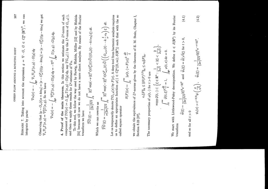
73

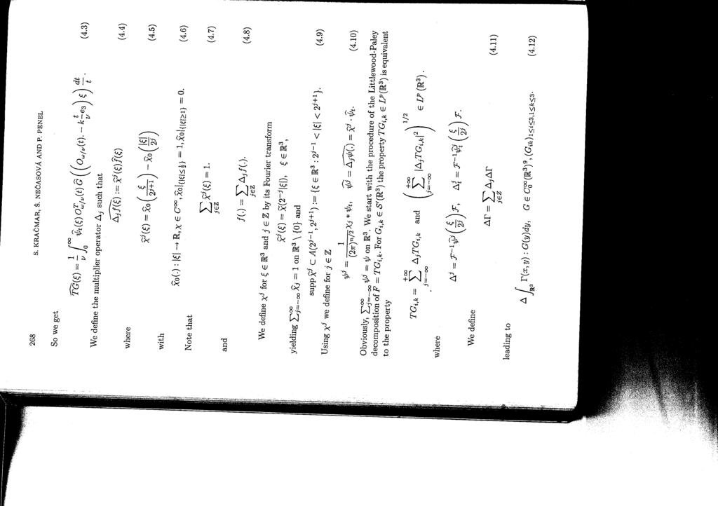
74

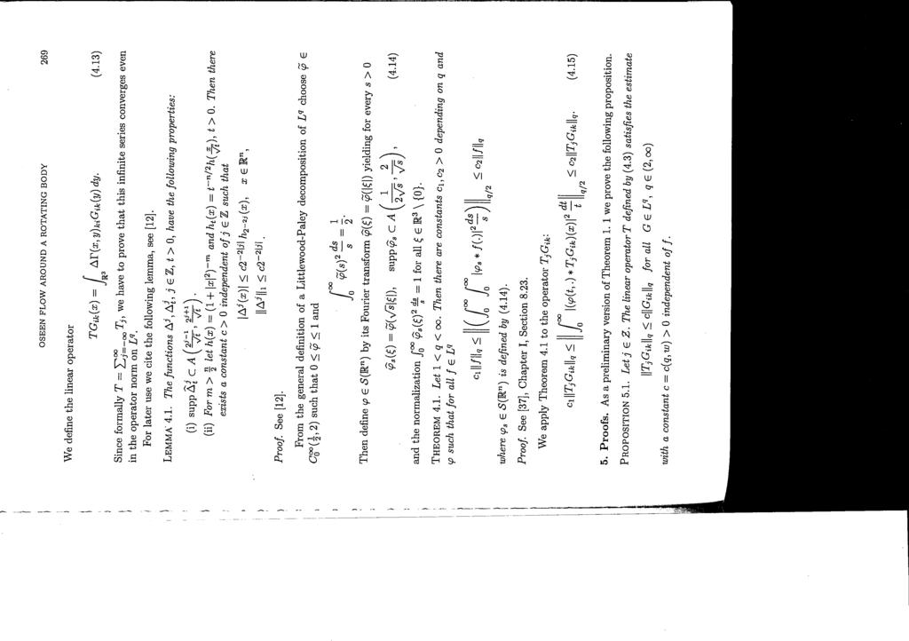
75

76

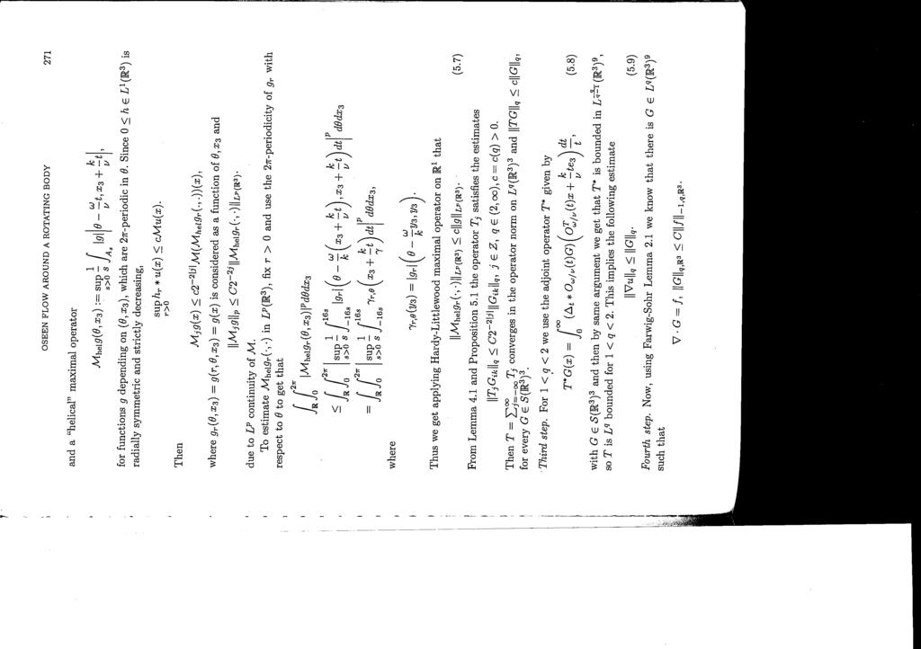
77

78

79

80

81

82

83 #21 The Mathematical Society of Japan J.Math.Soc.Japan Vol. 62, No. 1 21) pp doi: /jmsj/ Anisotropic L 2 -estimates of weak solutions to the stationary Oseen-type equations in 3D-exterior domain for a rotating body By Stanislav KRAČMAR, Šárka NEČASOVÁ and Patrick PENEL Received Jan. 4, 28) Revised Dec. 14, 28) Abstract. We study the Oseen problem with rotational effect in exterior three-dimensional domains. Using a variational approach we prove existence and uniqueness theorems in anisotropically weighted Sobolev spaces in the whole three-dimensional space. As the main tool we derive and apply an inequality of the Friedrichs-Poincaré type and the theory of Calderon-Zygmund kernels in weighted spaces. For the extension of results to the case of exterior domains we use a localization procedure. 1. Introduction Formulation of the problem. In a three-dimensional exteriordomain R 3, the classical Oseen problem [3] describes the velocity vector v and the associated pressure by a linearized version of the incompressible Navier-Stokes equations as a perturbation of v 1 the velocity at infinity; v 1 is generally assumed to be constant in a fixed direction, say the first axis, v 1 ¼jv 1 je 1. In the next we denote jv 1 j by k, and we will write the Oseen operator k@ 1 v. On the other hand it is known that for various flows past a rotating obstacle, the Oseen operator appears with some concrete non-constant coefficient functions, e.g. aðxþ ¼! x, where! is a given vector, see [17], [29]; in view of industrial applications aðxþ can also play the role of an experimental known velocity field, see [2]. This paper is devoted to the study of the following problem in for nonsolenoidal) vector function u ¼ uðxþ and scalar function p ¼ pðxþ: u þ k@ 1 u ð! xþru þ! u þrp ¼ f in ð1.1þ u! as jxj!1 div u ¼ g in ð1.2þ ð1.3þ u ¼ ð! xþ ke 1 ð1.4þ 2 Mathematics Subject Classification. Primary 35Q35; Secondary 35B45, 76D99. Key Words and Phrases. Oseen problem, rotating body, anisotropically weighted L 2 spaces.

84 24 S. KRAČMAR, Š.NEČASOVÁ and P. PENEL where! ¼ðe!; ; Þ is a constant vector,, k and e! aresomepositiveconstants, and f ¼ f ðxþ a given vector function, g ¼ gðxþ a given scalar function. We restrict ourselves to the assumption of compact support of g when is an exterior domain. The system arises from the Navier-Stokes system modelling viscous fluid around a rotating body which is moving with a given non-zero velocity in the direction of its axis of rotation. An appropriate coordinate transform and a linearization yield in the stationary case equations 1.1) and 1.2), for details see [3], [17]. The third term together with the fourth one the Coriolis force! u) in 1.1) arise from the influence of rotation of the body. Let us begin with some comments and relevant process of analysis of the problem 1.1) 1.4).. The governing equations of fluid motion are stationary and linear, but in unbounded domains the convective operators, k@ 1 and ð! xþr, cannot be treated as perturbations of lower order of the Laplacian.. The fundamental tensor similarly as the fundamental tensor to the Oseen problem) exhibits the anisotropic behavior in the three-dimensional space. To reflect the decay properties near the infinity we introduce the following weight functions: ðxþ ¼ ;ð Þ ¼ ð1 þ rþ ð1 þ "sþ ; ;" x with r ¼ rðxþ ¼jxj ¼ð P 3 i¼1 x2 i Þ1=2, s ¼ sðxþ ¼r x 1, x 2 R 3, "; >, ; 2 R. Discussing the range of the exponents and, the corresponding weighted spaces L q ðr 3 ; Þ give the appropriate framework to test the solutions to 1.1) 1.3). This paper is concerned with q ¼ 2. Let us mention also that belongs to the Muckenhoupt class A 2 of weights in R 3 if 1 <<1 and 3 <þ<3.. In this paper we will prefer the variational approach. To avoid the difficulties with the pressure part of the solution p we solve firstly the problem in R 3. Using the theory of Calderon-Zygmund integrals in corresponding weighted spaces, we determine the pressure p of the problem in R 3 to be from the same space as the right-hand side of 1.1). This first step cannot be done directly in an exterior domain. Then we apply the variational approach for the velocity part of the solution.. For the extension of the results to the case of exterior domains we use the localization procedure, see[22].

85 Anisotropic L 2 -estimates of solutions to Oseen-type equations Short bibliographical remarks. The weighted estimates of the solution to the stationary classical Oseen problem were firstly obtained by Finn in 1959, see [9]. The variational approach to the model equation u þ k@ 1 u ¼ f in an exterior domain in anisotropically weighted L 2 -spaces was applied by Farwig, see [1]. The same variational viewpoint has been also applied in [27], [28] bykračmar and Penel to solve the generic scalar model equation u þ k@ 1 u a ru ¼ f with a given nonconstant and, in general, non-solenoidal vector function a in an exterior domain. Both model equations are assumed with boundary conditions u ¼ and u! as jxj!1. Another common approach to study the asymptotic properties of the solutions to the Dirichlet problem of the classical steady Oseen flow is the use of the potential theory, i.e. convolutions with Oseen fundamental tensor and its first and second gradients for the velocity or with the fundamental solution of Laplace equation for the pressure): the L 2 -estimates in anisotropically weighted Sobolev spaces in R 3 were derived by Farwig [2], the L q -estimates in these spaces were proved in R 3 and R n by Kračmar, Novotný and Pokorný in [25] and [26], respectively. Different approach was used by Kobayashi and Shibata [21]. The fundamental solution to rotating Oseen problem in the time dependent case is known due to Guenther and Thomann, see [32], but, unfortunately, the respective stationary kernel does not seem to be of Calderon-Zygmund type. The Littlewood-Paley decomposition technique offers another approach for an L q -analysis: Thus, L q -estimates in non-weighted spaces were derived for the rotating Stokes problem by Hishida [17], by Farwig, Hishida, and Müller [5], and for the rotating Oseen problem in R 3 by Farwig [3], [4]. L q -estimates of the pressure and the gradient of the velocity for the exterior Stokes flow around a rotating body without translation were derived in [19]. L q -setting with non-integrable righthand side in non-homogeneous case was investigated by Kračmar, Nečasová and Penel in [24]. The Littlewood-Paley decomposition technique for L q -weighted estimates with anisotropic weight functions was used by Farwig, Krbec and Nečasová [7], [8]. Another approach based on the use of the non-stationary equations in both the linear and also non-linear cases is proposed by Galdi and Silvestre in [11], [12], [13], [14]. The last paper showed the existence of the wake region for the Navier-Stokes flow for small data. We would like also to mention that the problem was solved by the semigroup theory in L 2 -setting in particular by Hishida [18], and then the respective results were extended to L q case by Geissert, Heck and Hieber [15].

86 242 S. KRAČMAR, Š.NEČASOVÁ and P. PENEL 1.3. Basic notations and elementary properties. Let us outline our notations. Let S be the space of the moderate distributions in R 3.Letbe an exterior domain with a boundary of the class C 2,and bw m;q ðþ ¼fu 2 L 1 loc ðþ : Dl u 2 L q ðþ; jlj ¼mg with the seminorm juj m;q ¼ð P R jlj¼m jujq Þ 1=q. It is known that bw m;q ðþ is a Banach space and if q ¼ 2 the space bh m ðþ ¼ bw m;2 ðþ a Hilbert space), provided we identify two functions u 1, u 2 whenever ju 1 u 2 j m;q ¼, i.e. u 1, u 2 differ at most) on a polynomial of the degree m 1. Asusual,wedenoteby bw m;q ðþ the closure of C 1ðÞ in bw m;q ðþ. Let ðl 2 ð; wþþ 3 be the set of measurable vector functions f ¼ðf 1 ;f 2 ;f 3 Þ in such that Z kf k 2 2;; w ¼ jf j 2 wdx < 1: We will use the notation L 2 ; ðþ instead of ðl2 ð; ÞÞ3 and kk 2;; instead of kk ðl 2 ð; ÞÞ3. Let us define the weighted Sobolev space H 1 ð; ; 1 1 Þ as the set of functions u 2 L 2 ; ðþ with the weak i u 2 L 2 1 ; 1 ðþ. The norm of u 2 H 1 ð; ; 1 1 Þ is given by Z Z 1=2 kuk H 1 ¼ juj 2 dx þ jruj dx : ; ;1 1 As usual, H 1 ð; ; 1 1 Þ, will be the closure of C 1 ðþ in H 1 ð; ; 1 C 1 ðþ is ðc1 ðþþ3, and H 1 ð; ; 1 1 Þ will be the closure of C 1 H 1 ð; ; 1 1 Þ. For simplicity, we shall use the following abbreviations: 3 L 2 ; ðþ instead of L2 ; k k 2;;; instead of k k ðl2 ð; ÞÞ3 H 1 ; ðþ instead of H 1 ð; 1 1 ; Þ V ; ðþ instead of H 1 ð; 1 ; Þ V ; instead of H 1 ð; 1 ; Þ: 1 Þ,where ðþ in

87 Anisotropic L 2 -estimates of solutions to Oseen-type equations 243 We shall use these last two Hilbert spaces for, >, þ <3. Ifno confusion can occur, we omit the domain in the notation of the norm kk 2;;;. The notation H 1 ðþ and H 1 ðþ mean, as usual, the non-weighted spaces ðh 1 ð; 1; 1ÞÞ 3 and ðh 1 ð; 1; 1ÞÞ 3, respectively. As usual, omitting the domain in the notation of spaces will indicate that ¼ R 3,soe.g.H 1 ¼ H 1 ðr 3 Þ. Concerning the weight functions,wewillusetwonotations ðxþ and ðxþ taking the advantages of the following remark: ; ;" REMARK 1.1. Let us note that for ; ;" and for any 1; 2 ;" 1 ;" 2 > one has c min ; 2 ;" 2 ; 1 ;" 1 c max ; 2 ;" 2 ; c min ¼ minð1; ð 1 = 2 Þ Þminð1; ð" 1 =" 2 Þ Þ, c max ¼ maxð1; ð 1 = 2 Þ Þmaxð1; ð" 1 =" 2 Þ Þ. The parameters and " are useful to re-scale separately the isotropic and anisotropic parts of the weight function. We also use the notation of sets B R ¼fx 2 R 3 ; jxj Rg, B R ¼ fx 2 R 3 ; jxj Rg, R ¼ B R \, R ¼ B R \, B R 1 R 2 ¼ B R 1 \ B R2, R 1 R 2 ¼ B R 1 R 2 \, for positive numbers R, R 1, R Main results. In the first part of the paper chapters 2 4) we study the problem in R 3.Let us assume for a moment that pressure p is known. In solving the problem 1.1) 1.3) with respect to u and p by means of a pure variational approach, we shall deal with the following equation: Z Z jruj 2 wdx þ ðu rþu rwdx k Z juj 1 wdx R 3 R 3 2 R 3 1 Z Z Z juj 2 divðw! ½ xšþdx ¼ f u wdx rp u wdx 2 R 3 R 3 R 3 ð1.5þ as we get integrating formally the product of 1.1) by w u with w an appropriate weight function. First, let us note that divð ½! xšþ equals zero for w ¼.The left hand side can be estimated from below by: Z jruj 2 wdx þ 1 Z juj 2 jrwj 2 =w k@ 1 w dx: 2 R 3 2 R 3 ð1.6þ Because the term jrwj 2 =w k@ 1 w is known explicitly, we have the possibility to evaluate it from below by a small negative quantity in the form C 1 1 without any constraint in sðþ see Lemma 2.5).

88 244 S. KRAČMAR, Š.NEČASOVÁ and P. PENEL An improved weighted Friedrichs-Poincaré type inequality in H 1 ; is necessary. The obtained inequality allows us to compensate by the viscous Dirichlet integral the small negative contribution in the second integral of 1.6). We finally prove the existence of a weak solution 1.1) 1.3) in V ; by the Lax- Milgram theorem. The main results of the first part of the paper can be summarized in the following theorems parameters,,, " are specified in Section 1.3): THEOREM 1.2. Let >. There are positive constants R, c, c 1 depending on,,, " explicit expressions of these constants are given by Lemma 2.3, essentially c ¼ Oð" 2 þ 2 Þ and c 1 ¼ Oð" 1 1 Þ for and " tending to zero) such that for all v 2 H 1 ; Z kvk 2 2; 1; 1 c B R Z jrvj 2 dx þ c 1 B R jrvj 2 dx: ð1.7þ THEOREM 1.3 Existence and uniqueness). Let < 1, <y 1, f 2 L 2 þ1;, g 2 H1 loc such that rg kg e 1 þ gð! xþ 2L 2 þ1; ; y 1 will be given in Lemma 4.3. Then there exists auniqueweaksolutionfu; pg of the problem 1.1) 1.3) such that u 2 V ;, p 2 L 2 ; 1, rp 2 L2 þ1; and kuk 2; 1; þ kruk 2;; þ kpk 2;; 1 þ krpk 2;þ1; C kf k 2;þ1; þkrg kg e 1 þ g! ð x Þk 2;þ1; : In the second part of the paper chapters 5, 6) we extend the results of the first part onto exterior domains. THEOREM 1.4. Let R 3 be an exterior domain and <1, <y 1 ; y 1 isgiveninlemma4.3,f 2 L 2 þ1; ðþ, g 2 H 1 ðþ with supp g ¼ K and R gdx ¼. Then there exists a weak solution fu;pg of the problem 1.1) 1.4) such that u 2 V ; ðþ; p2 L 2 ; 1 ðþ, rp 2 L2 þ1;ðþ and kuk 2; 1; þ kruk 2;; þ kpk 2;; 1 þ krp C kf k 2;þ1; þkgk 1;2 þ! 2 þ! þ k 2 þ k : k 2;þ1; REMARK u and ru, our analysis did not catch any difference in the dependence of the parameters and. The reason appears inside the proofs of the Theorems 1.3 and 1.4 when we ask for the coercivity of the

89 Anisotropic L 2 -estimates of solutions to Oseen-type equations 245 bilinear form Qð; e Þ, testing equation 4.2) by u. On the other hand, we have no heuristic argument for not expecting better decay behavior 1 u like rp as in Farwig s result, see [2]. REMARK 1.6. The important feature of the Friedrichs-Poincaré type inequality is that we are able to evaluate its coefficients, precisely expressed in Lemma 2.3 separately near the obstacle and far from the obstacle. REMARK 1.7. For >, using these coefficients, negative values of the function F ; ð; Þ defined by the formula 2.13) can be compensated by the viscous Dirichlet integral; this analysis was not required in [2] becausef ; ð; Þ is positive when <. REMARK 1.8. The previous compensation cannot be associated with a large interval of positive values for : So, we receive the technical condition = < y 1. Using other type of weight functions characterized by some parameters, one can get another technical condition on these parameters. REMARK 1.9. We can improve the result from Theorem 1.4 removing the assumptions on g relative to its compact support and to its zero mean value: This will be the partial subject of a forthcoming paper. In the present paper, we have decided to use simply the approach by Girault-Raviart see Subsection 6.1) and the standard Bogovski s lemma in bounded domains, to get finally Corollary Friedrichs-Poincaré inequality. In this section we derive an inequality of the Friedrichs-Poincaré type in weighted Sobolev spaces. We also recall some necessary technical assertions, for more details see Kračmar and Penel [27]. PROPOSITION 2.1. For arbitrary ; and x 2 R 3, x 6¼ : ð x Þ 2 min ð 1; Þ" 1ð Þ: 1 x PROOF. We introduce ¼ minð; 1Þ in an explicit expression of : ¼ þ "s 1 þ "s 2 þ 2" s 1 þ r 1 þ r r þ 2ð 1Þ " r ð1 þ rþ "s 1 þ "s þ 2 2 ð1 þ "s Þ 1 r þ ð 1 þ Þ2 " r ð1 þ rþ 1 1 ;

90 246 S. KRAČMAR, Š.NEČASOVÁ and P. PENEL for r>. Wedenotethefivetermsinfgby T 1, T 2 ;...;T 5, and overwrite the previous relation as ¼f½T 1 þ T 4 ŠþT 2 þ½t 3 þð1 ÞT 5 Šþ T 5 g 1 1. Observing that T 5 2", the proposition is trivial. PROPOSITION 2.2. Let,, >, "> and >1. Then for x 2 R 3, jxj j 1 ð2"þ 1 jð 1Þ 1 : r ðxþ 2 2: 2 " ðþ Þ 2 1=2 ð Þ ð2.8þ 1=2 x Let,, >, "> and ð Þð2" Þ. Then for x 2 R 3, x 6¼ : r ðxþ 2 2: ð þ 2" Þ 2 1=2 ð Þ ð2.9þ 1=2 x PROOF. If ¼ and ¼ then both inequalities 2.8) and 2.9) are valid. Let us concentrate on the nontrivial cases: For r>, s 2½; 2rŠ, wehavethat@g=@s >, whereg is a function defined by relations: r ðxþ 2 2; ¼ gðsðxþ;rðxþþ 1=2 1=2 ðxþ gðs; rþ þ "s 1 þ r So, gðs; rþ is increasing as a function of s and Gr ðþmax gðs; rþ ¼g ð 2r; r Þ s2½;2rš þ 2" s r þ 22 " 2 1 þ r s 1 þ "s ¼ þ 2"r 1 þ r þ 4" þ 42 " 2 1 þ r 2 þ 1 þ 2"r ð Þ2 " ð2.1þ for >1 and r j 1 ð2"þ 1 jð 1Þ 1. So, inequality 2.8) is proved. To justify the second inequality 2.9), we observe that for the given values of,,, " and for r>, GðrÞ GðÞ. Next we derive an inequality of the Friedrichs-Poincaré type in the space H 1 ;. It is necessary for our aim to get expressions of constants in this inequality. It follows from Proposition 2.1. r :

91 Anisotropic L 2 -estimates of solutions to Oseen-type equations 247 LEMMA 2.3. Let, >, þ <3, >1. Let and " be arbitrary positive constants, such that ð Þð2" Þ. Then for all u 2 H 1 ; kuk 2 2; 1; 1 c krujb R k 2 2;; þ c 1 rujb R 2 2;; ; ð2.11þ where c ¼½ð þ 2"Þ=ð "ÞŠ 2, c 1 ¼½ð2Þ=ð"ÞŠ ½ð þ Þ=ð ÞŠ 2 and R j 1 ð2"þ 1 jð 1Þ 1. REMARK 2.4. Let us observe that if additionally <2" and 1 < 2"= þ =ð2"þ 1 then c c 1. PROOF OF LEMMA 2.3. Due to the density of C 1 in H 1 ; it is sufficient to prove the inequality for all u 2 C 1. From Proposition 2.1 it follows that for v 2 C 1 Z 2 " v dx v R 3 nb ZR 2 dx 3 nb Z ¼ 2 ðv rþv r Z@B dx þ v 2 r n ds R 3 nb Z " R 3 nb v dx þ 1 " Z þ v 2 r n Z jrv R 3 nb j 2 r 2 þ1 þ1 dx Hence, because the surface integral is a value of the order Oð 2 Þ,wehave: Z " v dx 1 Z jrvj 2 r R 3 2 þ1 " R 3 þ1 dx: ð2.12þ By means of the Cauchy-Schwarz inequality and from Proposition 2.2 with R j 1 ð2"þ 1 j=ð 1Þ we finally get 2.11). We will need some technical lemmas. Let us define F ; ðs; rþ by the relation: F ; ðs; rþ 1 1 r 2 = k@ 1 : The following lemma gives the evaluation of F ; ðs; rþ from below. ð2.13þ LEMMA 2.5. ;, k>. Then Let <, >1, <"ð1=ð2þþðk=þðð Þ= 2 Þ and

92 248 S. KRAČMAR, Š.NEČASOVÁ and P. PENEL F ; ðs; rþ 1 1 k" ð Þs k 1 þ k 1 ð2.14þ for all r> and s 2½; 2rŠ. PROOF. Expressing the function F ; ðs; rþ explicitly we get: F ; ðs; rþ ¼ þ "s 2" s 1 þ r r 22 " 2 kð1 þ "sþ r s þ k" ð1 þ rþ s r r : 1 þ r s 1 þ "s r For convenient use we subtract ð1 1 Þk"ð Þs from F ; ðs; rþ. Weobserve see Appendix A) that, for the given,, ",, for all,, k> and for r>, F ; ðs; rþ ð1 1 Þk"ð Þs F ; ð;rþ, which immediately gives inequality 2.14). 3. Uniqueness in R 3. In this section, we will start with the question about the unique weak solvability of the problem 1.1) 1.3) in ¼ R 3. The presented approach will be also used in the next section, in the proof of existence of a solution verifying solenoidality of the constructed function u. THEOREM 3.1 Uniqueness in R 3 ). Let fu;pg be a distributional solution of the problem 1.1) 1.3) with f ¼, g ¼ such that u 2 ch 1;2 and p 2 Lloc 2.Then u ¼ and p ¼ const. PROOF. From the condition u 2 c H 1;2 we get ru 2 L 2, u 2 L 6, u 2 S. Because divðð! xþru! uþ ¼ð! xþrdiv u ¼, we have 4p ¼. Hence, applying Laplacian and the Fourier transform we get 4 ð u þ k@ 1 u ð! xþru þ! uþ ¼ ; jj 2 jj 2 bu þ ik 1 bu ð! Þr bu þ! bu ¼ in S : Assuming the equation in cylindrical coordinates ð 1 ;; Þ, and denoting Tð Þ bv ¼ buð 1 ;; Þ, where T ð Þ ¼ 2 3 1; ; ; cos ð Þ; sin ð Þ5; ; sin ð Þ; cos ð Þ

93 Anisotropic L 2 -estimates of solutions to Oseen-type equations 249 we get n o jj bv þ½ð=e!þjj 2 þ iðk=e!þ 1 Šbv ¼ in S : ð3.15þ We will show that from this equation it follows that supp bv fg, and due to the definition of bv we will have also supp bu fg. This means that u is a polynomial of x 1, x 2, x 3.Becauseu 2 L 6 we get u ¼. Substituting into 1.1) we get rp ¼ and p ¼ const. So, we have to prove that for an arbitrary real vector function 2 C 1 ðr3 nfgþ defined for ½ 1 ; 2 ; 3 Š2R 3 we have hbv; i¼. If for each 2 C 1 ðr3 nfgþ there is a function 2 C 1 ðr3 nfgþ such jj 2 h þ ð=e!þjj 2 þ i ðk=e!þ 1 i jj 2 ¼ ð3.16þ then from 3.15) it follows: D E ¼ jj 2 bv þ½ð=e!þjj 2 þ i ðk=e!þ 1 Šbvg; D E ¼ ðjj 2 Þþ½ð=e!Þjj 2 þ i ðk=e!þ 1 Šðjj 2 Þ ¼ hbv; i: Hence, the proof of supp bv fg is reduced to the solvability of 3.16). First we note that it is sufficient to solve the þ ð=e!þjj 2 þ i ðk=e!þ 1 ¼ ð3.17þ because the division on the expression jj 2 defines the one-to-one correspondence of the space C 1 ðr3 nfgþ onto C 1 ðr3 nfgþ. Let us analyze the equation 3.17) in cylindrical coordinates ½ 1 ;; Š, where ¼ð2 2 þ 2 3 Þ1=2. For an arbitrary real vector function 2 C 1 ðr3 nfgþ defined for ½ 1 ; 2 ; 3 Š2R 3 we define fðtþ :¼ ð 1 ;cos t; sin tþ, a :¼ ð=e!þjj 2 þ iðk=e!þ 1, assuming e! >. Now, we will use the following technical proposition about the existence of a solution of an ordinary differential equation in a space of periodical functions and later also in the proof of existence of a solution of the problem for checking solenoidality of a constructed solution, see the proof of Theorem 4.4): PROPOSITION 3.2. Let a 2 C, Re a>. Letf 2 C 1 ðrþ be a 2-periodical complex function. Then there is unique 2-periodical solution g 2 C 1 ðrþ of the equation

94 25 S. KRAČMAR, Š.NEČASOVÁ and P. PENEL g þ ag¼ f and the solution g can be expressed in the following form: Z g ð Þ ¼ e 2a Z e at f þ ð tþdt ¼ e a e at ft ðþdt: 1 Proof of the proposition follows from standard computations. Using the Proposition 3.2 we get the solution of 3.17) in the form ð 1 ;; Þ ¼ exp 2 e! jj2 þ i k e! Z 2 exp e! jj2 þ i k e! 1 t ð ;cosðt þ Þ;sinðt þ ÞÞdt: It is easy to see that function as the function of ½ 1 ; 2 ; 3 Š is infinitely differentiable with respect to these variables and 2 C 1 ðr3 nfgþ. Finally we put ¼ =jj Existence of a solution in R 3. In this section we will construct a weak solution of the problem 1.1) 1.3) Existence of the pressure in R 3. If there exist distributions u;p satisfying u þ k@ 1 u ð! xþru þ! u þrp ¼ f in R 3 then pressure p satisfies the equation div u ¼ g in R 3 4 p ¼ div F; where F ¼ f þ rg kg e 1 þ gð! xþ; ð4.18þ because divðð! xþru! uþ ¼ð! xþrdiv u ¼ div½gð! xþš. Let E be the fundamental solution of the Laplace equation, i.e. E ¼ 1=ð4rÞ. Assuming firstly F 2 C 1 we have p ¼ E? div F and rp ¼rE? div F and so, p ¼rE? F and rp ¼r 2 E? F. It is well known that both formulas can be extended for F 2 L 2 þ1; with <<1and 2 <þ<2 the last convolution rp ¼r 2 E? F due to the fact that r 2 E is the singular kernel of the Calderon- Zygmund type and that þ1 belongs to the Muckenhoupt class of weights A 2 ), see [2, Theorem 3.2, Theorem 5.5], [26, Theorem 4.4, Theorem 5.4], where the

95 Anisotropic L 2 -estimates of solutions to Oseen-type equations 251 theorems are formulated for the pressure part P of the fundamental solution of the classical Oseen problem, so P ¼rE and rp ¼r 2 E.ForF 2 L 2 þ1; we get p 2 L 2 ; 1 and rp 2 L2 þ1;, and there are positive constants C 1;C 2 such that the following estimates are satisfied: kpk 2;; 1 C 1 kfk 2;þ1; ; krpk 2;þ1; C 2 kfk 2;þ1; ð4.19þ REMARK. Another possibility of construction of the pressure is the use of Hörmander-Michlin multiplier theorem.bothtechniquescanbeusedinl 2 -as well as in L q -framework to get an estimate of rp The problem in B R. We will study in this section the existence of a weak solution of the following problem in a bounded domain B R, pressure p is assumed here to be known, the right hand side f rp ¼ e f 2 L 2 þ1; : u þ k@ 1 u ð! xþru þ! u ¼ e f in B R ð4.2þ u ¼ R : ð4.21þ We show the existence of a weak solution u R 2 H 1 ðb R Þ. Following 1.5), 1.6) again with w ¼, 2ð; 1Š, using notation 2.13), let us introduce a continuous bilinear form e Qð; Þ on H 1 ðb R ÞH 1 ðb R Þ: Z eq ðu; vþ ¼ ru : r v B R Z þ ð! xþru v B R Z dx þ k dx 1 u v dx B R Z ð! uþ v Z eq ðv; vþ 2 1 jrvj 2 dx þ 2 1 v B R ZB 2 F ; ðs; r; R LEMMA 4.1. B R Þ 1 dx; 1 dx: ð4.22þ Let < 1. Then,forall e f 2 L 2 1; ðb R Þ, " < ð1=2þðk=þ ð1= Þ, ;" ;", there exists unique u R 2 H 1 ðb R Þ such that for all v 2 H 1 ðb R Þ. Z eq ðu R ; vþ ¼ e f v dx: ð4.23þ B R PROOF. Bilinear form Q e is coercive, i.e. there exists a constant C R > such that Qðv; e vþ C R kvk 2,wherekkis the norm in the space H 1 ðb R Þ. Indeed, we get

96 252 S. KRAČMAR, Š.NEČASOVÁ and P. PENEL eq ðv; vþ Z jrvj 2 2 dx þ 1 Z v 2 F ; ðs; rþ 1 B R 2 1 dx B R Because " < ð1=2þðk=þð1= Þ there is a constant satisfying all previous conditions and additionally " ð1=2þðk=þð1= Þ. Because ¼ we get from Lemma 2.5 Z v 2 F ; ðs; rþ 1 1 B R Z eq v; v ð Þ 2 dx 1 1 k" 2 v ZBR sdx; jrvj 2 dx þ 1 B R Z k" v ð " sþdx: B R Using Lemma 2.3 and Remark 2.4 we derive: eq ðv; vþ Z jrvj 2 4 dx þ Z B R 16 "2 2 v dx B R þ Z k" v ð " sþdx B R min 1; 1 4 "2 2 ; 2 k " Z Z jrvj 2 dx þ v 2 1 dx B R B R Z eq ðv; vþ C R jrvj ZB 2 dx þ v 2 dx ¼ C R kvk 2 ; R B R ð4.24þ ð4.25þ where C R ¼ð=4Þð1 1 Þminf1; " 2 2 =4; 2ðk=Þ" gð1 þ " RÞ. Using Lax- Milgram theorem we get that there is u R 2 H 1 ðb R Þ such that 4.23) is satisfied. REMARK 4.2. An arbitrary function 2 H 1 ðb R Þ can be expressed in the form ¼ v,wherev 2 H 1 ðb R Þ. Therefore for all 2 H 1 ðb R Þ Z Qðu R ; Þ ¼ e f dx; B R where by the definition Qðu R ; Þ Qðu R ; v Þ e Qðu R ; vþ. ð4.26þ

97 Anisotropic L 2 -estimates of solutions to Oseen-type equations Uniform estimates of u R in R 3. Our next aim is to prove that the weak solutions u R of 4.23) are uniformly bounded in V ; as R!þ1. Let y 1 be the unique real solution of the algebraic equation 4y 3 þ 8y 2 þ 5y 1 ¼. Itiseasytoverifythaty 1 2ð; 1Þ. We will explain later, why the control of = by y 1 is necessary. LEMMA 4.3. Let <1, <y 1, e f 2 L 2 þ1;.then,asr!þ1,the weak solutions u R of 4.23) given by Lemma 4.1 are uniformly bounded in V ;. There is a constant c>, which does not depend on R such that Z R 3 Z ~u 2 R 1 dx þ jr ~u R j 2 dx c e f R ZR 2 þ1 dx ð4.27þ 3 3 for all R greater than some R >, ~u R being extension by zero of u R on R 3 n B R. PROOF. First, we derive estimate of u R on a bounded subdomain B R B R ; ThechoiceofR will be given in the next part of the proof. Our aim is to get an estimate with a constant not depending on R. Let us substitute v ¼ u R into 4.23).Hence,wegetfrom4.24): Z Z eq ðu R ; u R Þ ¼ e fur dx C 1 B R jru R B R Z j 2 dx þ u 2 R 1 B R with the constant C 1 > stated in 4.24). Let R be some fixed positive number such that <R <R.Weget Z B R Z jru R j 2 dx þ B R u 2 R 1 dx ; dx C 2 e f ju R j ZB dx; ð4.28þ R where the constant C 2 ¼ C 1 1 ð1 þ " R Þ ð1 þ " 2 R Þ j j depends on k,,,,, ", R,, but does not depend on R. Now, we are going to derive an estimate of u R on domain B R.Usingthetest function ¼ u R ¼ u Rð1 þ rþ ð1 þ "sþ 2 H 1 ðb R Þ in 4.26) we get after integration by parts: Z jru R j 2 dx þ ðu R ru R Þr B R ZB dx k R 2 Z ¼ e fur dx: B R Z B R u 2 1 dx

98 254 S. KRAČMAR, Š.NEČASOVÁ and P. PENEL So, we get for some >1: Z jru R j 2 2 dx þ 1 Z u 2 R B R 2 F ;ðs; rþ 1 1 dx e f ju R j B R ZB dx: R Let R j 1 ð2"þ 1 jð 1Þ 1. Using Lemma 2.5 with <, " ð1=ð2þþ ðk=þðð Þ= 2 Þ) and Lemma 2.3 with <2"), the second term in the previous estimate can be evaluated from below: Z u 2 R F ;ðs; rþþ 1 1 dx B R k 1 þ 2 k þ 1 1 þ 2 Z " Z k" ð Þ u 2 R 1 B R R B R R jru R j 2 dx 1 sdx 2C 4 Z B R jru R j 2 dx: Denote C 5 ¼ kð1 þ =kþð=ð"þþðð þ Þ=ð ÞÞ 2. It is clear that C 5 =ð2 2 Þ <=ð2 Þ if 1 þ =k i.e. ðk=þðð 1ÞÞ=ðÞ) and ð1=ð2 4 ÞÞ ð=kþðð Þ=ð þ ÞÞ 2 ".Wehave Z jru R j 2 2 dx þ 1 B R k" ð Þ Z Z C 6 u 2 R 1 1 dx C 7 ru R B R B R Z j j 2 dx ZB R e f u 2 R 1 1 sdx B R ju R j dx: We use now relation 4.28) in order to estimate the integrals computed on the domain B R. Before using the mentioned inequality we should re-scale it with respect to new values ";, see Remark 1.1. The new constant in 4.28) after rescaling we denote C 2. Z jru R j 2 B R Z Z dx þ k" ð Þ u 2 R 1 1 sdx C 8 B R B R e f ju R j dx; where C 8 ¼f1 þ C 2 maxðc 6;C 7 Þg 2 ð1 1 Þ 1. We use Lemma 2.3 and Remark 2.4. So, if <2" and 1 < 2"= þ =ð2"þ 1 we get 2 " 2 Z þ 2" u 2 R 1 1 dx B R 2 Z B R jru R j 2 dx;

99 So we get Z 2 B R jru R j 2 dx þ 2 þ k" ð Þ Z " 2 Z þ 2" Z u 2 R 1 1 sdx C 8 B R u 2 R 1 1 dx B R B R e f ju R j dx: Z Z Z jru R j 2 dx þ 2 u 2 R 1 1 dx þ 2" u 2 R 1 1 sdx B R B R B R Z Z ¼ jru R j 2 dx þ 2 u 2 R 1 dx C 1 e f ju R j B R B R ZB dx; R C 9 ¼ minð=ð2þ; ð=ð2þþ ð "=ð þ 2"ÞÞ 2, kð Þ=2Þ and C 1 ¼ C 8 =C 9. We have also: Z B R e f ju R j dx t Z 2 So, if we choose t ¼ 2 C1 1 Z jru R B R Anisotropic L 2 -estimates of solutions to Oseen-type equations 255 u 2 R 1 B R then we get: j 2 dx þ Z u 2 R 1 B R dx þ 1 2t Z dx c Z R 3 B R e f 2 þ1 dx e f 2 þ1 dx: It can be easily shown that the all conditions on,,, ", used in the proof are compatible if <y 1, see Appendix B The problem in R 3. Let y 1 be the same as in Lemma 4.3. THEOREM 4.4 Existence and uniqueness in R 3 ). Let <1, < y 1, f 2 L 2 þ1;, g 2 H1 loc such that rg kg e 1 þ gð! xþ 2L 2 þ1;. Then there exists a unique weak solution fu; pg of the problem u þ k@ 1 u ð! xþru þ! u þrp ¼ f in R 3 ; ð4.29þ such that u 2 V ;, p 2 L 2 ; 1, rp 2 L2 þ1; and kuk 2; 1; þ kruk 2;; þ kpk 2;; 1 þ krpk 2;þ1; C kf k 2;þ1; þ krg kg e 1 þ g! ð xþ div u ¼ g in R 3 ð4.3þ k 2;þ1; : ð4.31þ

100 256 S. KRAČMAR, Š.NEČASOVÁ and P. PENEL PROOF. The uniqueness of the solution follows from Theorem 3.1, and we now justify the existence. Let p be the same as in Subsection 4.1. Let fr n g be a sequence of positive real numbers, converging to þ1. Let u Rn be the weak solution of 4.2), 4.21) on B Rn. Extending u Rn by zero on R 3 n B Rn to a function ~u n 2 V ; we get a bounded sequence f ~u n g in V ;. Thus, there is a subsequence ~u nk of ~u n with a weak limit u in V ;. Obviously, u is a weak solution of 4.29) and Z kuk 2 2; 1; þ kruk2 2;; lim inf k2n c e f 2 þ1 R 3 Z ~u 2 n k 1 dx þ Z jf rp R 3 dx ¼ c R 3 jr ~u nk j 2 dx j 2 þ1 dx: Taking into account also relation 4.19) we get 4.31). Let us also check that for u the equation 4.3) is satisfied. Let us mention that u 2 H loc 2 because f rp 2 L2 þ1;. So, computing the divergence of 4.29), we get divu ð Þþk@ 1 ðdiv uþ ð! x in the distributional sense. From 4.18) we have þ k@ 1 ð! xþr ¼ Þrðdiv uþ ¼ div f 4p ð4.32þ for ¼ div u g 2 L 2 ; L2. Using Fourier transform we get jj 2 þ ik 1 b ð! Þr b ¼ in S : Assuming b in cylindrical coordinates ½ 1 ;; Š, ¼ð 2 2 þ 2 3 Þ1=2,wecanoverwrite the equation in the form: h b þ ð=e!þjj 2 þ i ðk=e!þ 1 b ¼ : Using the same approach as in the proof of the uniqueness Theorem 3.1 we prove that supp b fg. The proof of this fact is reduced to the solvability of the equation 3.17) which was proved for arbitrary 2 C 1ðR3 nfgþ in the proof of Theorem3.1.So,bythesameprocedurewederivethat is a polynomial in R 3 and because 2 L 2 we get, i.e. 4.3).

101 Anisotropic L 2 -estimates of solutions to Oseen-type equations Uniqueness in an exterior domain R 3. The last two sections are devoted to the problem in an exterior domain. We start with the question of uniqueness. The uniqueness theorem proved in this section together with the uniqueness theorem in R 3 from Section 3 will be used in thenextsectionintheproofoftheexistenceofasolutioninanexteriordomain,in the localization procedure. The homogenous Dirichlet boundary condition for u in the next theorem follows from the assumption u 2 V ; ðþ. THEOREM 5.1. Let fu;pg be a distributional solution of the problem 1.1) 1.3) with f ¼ and g ¼ such that u 2 V ; ðþ and p 2 L 2 1;ðÞ. Thenu ¼ and p ¼. PROOF. Let ¼ ðzþ 2C 1 ðh; þ1þþ be a non-increasing cut-off function such that ðzþ 1 for z<1=2 and ðzþ for z>1. Let j j3. Let R R ðxþ ðjxj=rþ. We have jr R j3=r and j@ 1 R j3=r for x 2 R 3, R=2 jxj R. LetfR j g2r be an increasing sequence of radii with the limit þ1. Sowehavethatu j u Rj 2 H 1 ðþ, andfu j g is a sequence of functions with limit u in the space V ; ðþ. Using the non-solenoidal) test functions ¼ u 2 R j ¼ u j Rj 2 H 1 ðþ for equation 1.1) we get: Z Z ru : r u 2 R j dx þ 1 u u 2 R j dx Z Z þ ð! xþru u 2 R j dx þ rp u 2 R j dx ¼ : ð5.33þ Using in 5.33) relation ru : rðu 2 R j Þ¼jru j j 2 r Rj r Rj juj 2, integrating by parts, we get after some evident rearrangements Z ru j 2 dx 1 Z div ð! xþu j 2 dx 2 k Z juj 1 2 R 2 j dx 1 Z juj 2 ð! xþr 2 R 2 j dx Z Z r Rj 2 juj 2 dx pu r 2 R j dx ¼ : Z ru j 2 dx C Z Rj=2 Rj Z juj 2 r 1 dx þ Rj=2 Rj jpjjujr 1 dx u 2 L 2 1; ðþ, p 2 L2 1; ðþ, pu 2 L1 1; ðþ. So,forj!1we get R jruj2 dx. Hence, the function ru ¼ a.e. in, and this means u is a constant a.e. in.! :

102 258 S. KRAČMAR, Š.NEČASOVÁ and P. PENEL From u 2 L 2 1;ðÞ it follows that u ¼ a.e. in. Using now an arbitrary test function for equation 1.1), we get R rpdx ¼. So, the function rp ¼ a.e. in, andthismeansp is a constant a.e. in. Fromp 2 L 2 1;ðÞ it follows that p ¼ a.e. in, and the uniqueness is proved. 6. Existence of solution in exterior domains. In this section we assume problem 1.1) 1.4) in an exterior domain. First we assume the case of the homogenous Dirichlet boundary condition 6.1. Homogenous Dirichlet boundary conditions. Function g is assumed to be zero, and f ¼ div F with F 2 C 1ðÞ9. We will prove that the problem has a weak solution fu;pg2ch 1 ðþl2 locðþ. So we assume the following sequence of problems on domains R ¼ B R \ : u R þ k@ 1 u R þ ð! xþru R! u R þrp R ¼ Div F in R ð6.34þ div u R ¼ in R ð6.35þ u R ¼ R ð6.36þ Following Girault-Raviart [16], we formulate each problem in the following mixed variational form: To find fu R ;p R g2w R R, such that for all v 2 W R, 2 R : aðu R ; v where W R ¼ ch 1 ð RÞ, R ¼ kk WR ¼krk 2, kk R ¼kk 2,and a; ð Þþbðv; p R Þ ¼ hdiv F; vi ð6.37þ bðu R ;Þ ¼ ; ð6.38þ n 2 L 2 ð R Þ; R o R dx ¼ Z Z Þ ¼ r r dx þ 1 dx R R Z þ ½ð! xþr! Š dx R Z b; ð Þ ¼ div dx: R with usual norms These bilinear forms are continuous on W R W R and W R R, respectively. It is easy to see that að; Þ kk 2 W R, and it is known that sup v2w R ð; div vþ C kk jvj R W R

103 Anisotropic L 2 -estimates of solutions to Oseen-type equations 259 for some C ¼ C ðrþ >. Hence, there exists a weak solution fu R ;p R g of the problem and ku R k W R þkp R k R C 1 kdiv Fk 1 for some C 1 ¼ C 1 ðrþ >. Testing now 6.37) by v ¼ u R we get: Z Z jru R j 2 dx ¼ R R Z ðdiv FÞu R dx ¼ R F : ru R dx kfk 2 kru R k 2 kru R k 2 1 kfk 2 : ð6.39þ Since the a priori estimate 6.39) is available, where u R is understood as its extension by setting zero in n R, there exists u 2 ch 1 ðþ and a sequence fr n g!1so that u Rn * u weakly in ch 1 ðþ as n!1. Let us show that div u ¼ in L 2 ðþ. From the same inequality follows the weak convergence of div u Rn in L 2 ðþ. From 6.38) we get div u Rn C n on Rn for some real constant C n depending on n. In spite of 6.39) we get that the weak limit of div u Rn is zero in L 2 ðþ. Finally, for all 2 C 1 ðþ with div ¼ we have from 6.37) after R n!1 hlu Div F; i ¼ ; Lu uþk@ 1 u þ ð! xþru! u: By a result of de Rham, there is a distribution p such that rp ¼ Lu Div F in D ðþ. Because the right-hand side belongs to H 1 ð R Þ for every sufficiently large R> we have that p 2 L 2 ð R Þ and so, p 2 L 2 loc ðþ. Nowweusethefollowing LEMMA 6.1 Kozono and Sohr [22, Lemma 2.2, Corollary 2.3]). Let R n ðn 2Þ be any domain and let 1 <q<1. For all g 2 W b 1;q ðþ, there is G 2 L q ðþ n such that div G ¼ g; kgk q; Ckgk 1;q; with some C>. As a result, the space fdiv G; G 2 C 1 ðþn g is dense in bw 1;q ðþ. Hence, we get the existence of solution fu;pg2ch 1 ðþl2 locðþ for an arbitrary function e f 2 ch 1 ðþ. For the extension of Theorem 4.4 to the case of an exterior domain we use the localization procedure, see [22]. Let now f 2 L 2 þ1;ðþ. We define for an arbitrary R>:

104 26 S. KRAČMAR, Š.NEČASOVÁ and P. PENEL f R ¼ f ; x 2 R ; x 2 n R. It can be shown that f R belongs to ch 1 ðþ\l 2 þ1;ðþ. By use of cut-off function we decompose the solution fu;pg of the problem 1.1) 1.4) with the homogenous Dirichlet boundary condition) on the solution of a problem in R 3 and the solution of a Stokes problem in a bounded domain: u ¼ U þ V where U ¼ð1 Þu, V ¼ u p ¼ þ where ¼ð1 Þp, ¼ p; where 2 C 1, supp B 1 such that 1 on B, < < 1 <so that R 3 n B. We get that fu;g is a weak solution of the modified Oseen problem in R 3 4 U þ k@ 1 U ð! xþru þ! U þr ¼ Z 1 ð6.4þ div U ¼ r u ð6.41þ and fv ;g is weak solution of the Stokes problem in a bounded domain 4 V þr ¼ Z 2 in ð6.42þ div V ¼r u in ð6.43þ V ¼ ð6.44þ where the right-hand sides are given by Z 1 and Z 2. Z 1 ¼ 2r ru þ u 4 k@ 1 u þðr ð! xþþu r p þ ð1 Þf R ; Z 2 ¼ 2r ru u 4 þ k@ 1 u þ þr p þ f R : ½ð! xþru! uš Let us mention that Z 1 2 L 2 þ1;ðþ. To solve the Stokes problem on the bounded domain we use the following lemma, see [22]: LEMMA 6.2 The Stokes problem on a bounded domain). bounded domain of R n, n 2, ofclassc mþ2, m. Forany Let be a f 2 W m;q ðþ; g 2 W mþ1;q ðþ; v 2 W mþ2 1=q;q ð@þ;

105 Anisotropic L 2 -estimates of solutions to Oseen-type equations <q<1, with Z Z v n ds ¼ ð6.45þ there exists one and only one solution fv ;g to the Stokes system 4V þr ¼ f in div V ¼ g in V ¼ v such that V 2 W mþ2;q ðþ, 2 W mþ1;q ðþ and kv k mþ2;q þk k mþ1;q c kf k m; q þkv k mþ2 1=q; q þkgk mþ1;q ; ð6.46þ where ¼jj 1 R dx and c ¼ cðm; n; q; Þ. Furthermore, for of class C 2, for every f 2 W 1;q ðþ; g 2 L q ðþ; v 2 W 1 1=q;q ð@þ; 1 <q<1, with 6.45) there exists one and only one q-generalized solution fv ;g to the Stokes system such that V 2 W 1;q ðþ, 2 L q ðþ and the estimate 6.46) is valid with m ¼ 1. From the results about the existence and uniqueness of solutions of the Oseen problem in R 3 6.4), 6.41), i.e. from Theorem 4.4 and Theorem 3.1 it follows, that a solution fu;g is subject of the estimate 4.31), with f and g replaced by Z 1 and r u, respectively. Using also the respective results in a bounded domain for 6.42) 6.44), see Lemma 6.2 with m ¼ and bounded domain,we get the following lemma for an exterior domain: LEMMA 6.3. Let R 3 be an exterior domain and < 1, <y 1 ; y 1 is given in Lemma 4.3. Then there exists a weak solution fu;pg of the problem 1.1) 1.3) with the homogenous Dirichlet boundary condition, f :¼ f R and g ¼, such that u 2 V ; ðþ, p 2 L 2 ; 1 ðþ, rp 2 L2 þ1;ðþ and kuk 2; 1; þ kruk 2;; þ kpk 2;; 1 þ krpk 2;þ1; C 1 kf R k 2;þ1; þ kuk 1;2; A þ kpk ;2; ; ð6.47þ where A :¼ B n B =2, and constant C 1 does not depend on R.

106 262 S. KRAČMAR, Š.NEČASOVÁ and P. PENEL Now, we would like to show that the preceding estimate is valid with another constant) also if we add to the left-hand side the L 2 -norm of second gradient of u on some compact subset of. Taking into account the assertion of Lemma 6.2 for m ¼, wegetthatu2w 2;2 1;2 locðþ, p 2 Wloc ðþ. Multiplying the relation 1.1) 1.4) in an exterior domain with g ¼ and the homogenous Dirichlet boundary condition byu and integrating over the compact set K 1 with A K 1, weget kuk 2;K1 C 2 kuk 2;K1 þkruk 2;K1 þkpk 2;K1 þkrpk 2;K1 þkf R k 2;K1 : ð6.48þ Using 6.47), 6.48) and the known relation kr 2 uk 2;K c kuk 2;K1 þkruk 2;K1 with A K K 1,weget COROLLARY 6.4. In conditions of Lemma 6.3 the following estimate is valid and constant C does not depend on R: kuk 2; 1; þ kruk 2;; þ r 2 u 2; A þ kpk 2;; 1 þ C kf R k 2;þ1; þ kuk 1;2; A þ kpk ;2; krpk 2;þ1; : ð6.49þ Now, we will prove that the estimate 6.49) is valid without the right-hand side terms containing u and p with constant c which does not depend on R, i.e. we will prove: kuk 2; 1; þ Let us define the norms: kruk 2;; þ r 2 u 2; A þ kpk 2;; 1 þ krpk 2;þ1; ckf R k 2;þ1; ð6.5þ kðv;qþk ð1þ :¼kvk 1;2;A þkqk ;2; kðv;qþk ð2þ :¼kvk 2; 1; þkrvk 2;; þkr 2 vk 2; A þkqk 2;; 1 þkrqk 2;þ1; : For the corresponding Hilbert spaces H 1, H 2,wehaveH 2,!,! H 1.Letusassume that the estimate 6.5) is not true. This means that there is a sequence of

107 Anisotropic L 2 -estimates of solutions to Oseen-type equations 263 n o 1 functions f ðkþ R k with R k!þ1, a sequence of corresponding solutions k¼1 fðu k ;p k Þg 1 k¼1 and a sequence of constants fc kg 1 k¼1!1such that: 1 ku k k 2; 1; þkru k k 2;; þkr 2 u k k 2; A þkp k k 2;; 1 þkrp k k 2;þ1; kðu k ;p k Þk ð2þ c k f ðkþ : 2;þ1; n So we get f ðkþ R k R k 2;þ1; ok!. Thesequencefðu k;p k Þg 1 k¼1 is bounded in the norm kk ð2þ, so there is a subsequence of this sequence we will denote this subsequence using the same notation) with the weak limit ðu;pþ in the corresponding Hilbert space H 2.So,ðu;pÞ is a solution of the problem with the zero right-hand side. Due to uniqueness given by Theorem 5.1 we conclude that kðu;pþk ð2þ ¼. Because H 2,!,! H 1, we have kðu u k ;p p k Þk ð1þ!. From Corollary 6.4 we also get kðu u k ;p p k Þk ð2þ! ; i.e. fðu k ;p k Þg 1 k¼1 converges strongly in H 2. Because kðu k ;p k Þk ð2þ ¼ 1 for k 2 N, so we also get kðu;pþk ð2þ ¼ 1. This is the contradiction. So, we proved the following THEOREM 6.5. Let R 3 be an exterior domain and <1, < y 1 ; y 1 isgiveninlemma4.3,f 2 L 2 þ1;ðþ. Then there exists a weak solution fu;pg of the problem 1.1) 1.3) with the homogenous Dirichlet boundary condition g ¼, suchthatu 2 V ; ðþ, p 2 L 2 ; 1 ðþ, rp 2 L2 þ1;ðþ and kuk 2; 1; þ kruk 2;; þ kpk 2;; 1 þ krpk 2;þ1; Ckf k 2;þ1; : REMARK 6.6. The used contradiction argument is based on a subtle choice n of the sequence f ðkþ R k ok with R k!þ1. We cannot construct a contradiction separately for f R with fixed R because then the constant c in 6.5) may depend on R Non-homogenous cases. In this subsection we take into account the non-homogenous Dirichlet boundary condition and the non-homogenous continuity equation. We can prove the following extension of Theorem 6.5 for the case g 6¼ : COROLLARY 6.7. Let R 3 be an exterior domain and <1, <y 1 ; y 1 is given in Lemma 4.3, f 2 L 2 1;2 þ1;ðþ, g 2 W ðþ,withsupp g ¼

108 264 S. KRAČMAR, Š.NEČASOVÁ and P. PENEL K and R gdx ¼. Then there exists a weak solution fu;pg of the problem 1.1) 1.3) with the homogenous boundary condition such that u 2 V ; ðþ, p 2 L 2 ; 1 ðþ, rp 2 L2 þ1;ðþ and kuk 2; 1; þ kruk 2;; þ kpk 2;; 1 þ krpk 2;þ1; C kf k 2;þ1; þkgk 1;2 : First of all let us recall the lemma which will be used for the extension of our results to the case with nonzero divergence: LEMMA 6.8 M. E. Bogovski, G. P. Galdi, H. Sohr). Let R n, n 2,bea bounded Lipschitz domain, and 1 <q<1, n 2 N. Then for each g 2 W k;q ðþ with n R W gdx ¼, thereexistsg 2 kþ1;q ðþ satisfying div G ¼ g; kgk ðw kþ1;q ðþþ n Ckk g W k;q ðþ with some constant C ¼ Cðq; k; Þ >. For the proof and further references see e.g. [31, Lemma 2.3.1]. PROOF OF COROLLARY 6.7. Using Lemma 6.8 we find G 2 W 2;2 ðþ, supp G K, where K is a bounded Lipschitz domain being contained in "-neighbourhood K " of compact set K for an arbitrary ">, div G ¼ g, kgk 2;2 Ckgk 1;2.Wechoose" such that K ". Let us assume the following problem U þ k@ 1 U ð! xþru þ! U þrp ¼ F in div U ¼ in with the homogenous Dirichlet boundary condition for U, whereu ¼ u G, F ¼ f þ G k@ 1 G þð! xþrg! G. The assertion of Corollary 6.7 follows from Theorem 6.5. Now we justify our third main theorem. THEOREM 6.9. Let R 3 be an exterior domain and <1, <y 1 ; y 1 is given in Lemma 4.3, f 2 L 2 1;2 þ1;ðþ, g 2 W ðþ,withsupp g ¼ K and R gdx ¼. Then there exists a weak solution fu;pg of the problem 1.1) 1.4) such that u 2 V ; ðþ, p 2 L 2 ; 1 ðþ, rp 2 L2 þ1;ðþ and

109 Anisotropic L 2 -estimates of solutions to Oseen-type equations 265 kuk 2; 1; þ kruk 2;; þ kpk 2;; 1 þ krpk 2;þ1; C kf k 2;þ1; þkgk 1;2 þ! 2 þ! þ k 2 þ k : PROOF. Let >be such that R 3 n B =2. Let ¼ ðzþ 2C 1 ðh; þ1þþ be a non-increasing cut-off function such that ðzþ 1 for z<1=2 and ðzþ for z>1. Let j j3. Let ðxþ ðjxj=þ. We have jr j3= and j@ 1 j3= for x 2 R 3, =2 jxj. Let us define eu ¼ u ½ð! xþ ke 1 Š ðxþ. Then function ðeu;pþ satisfies to 1.1) 1.3) with the homogenous Dirichlet boundary condition, where f 2 L 2 þ1;ðþ is replaced by some another function e f 2 L 2 þ1; ðþ, and g by another function eg 2 C 1ðÞ with supp eg ¼ K [ A, A :¼ B n B =2 and Z egdx ¼ : So, using now Corollary 6.7 we get the assertion of Theorem 6.9. Appendix A. Relation 2.14) follows from an estimate of the derivative of F F F ;ðs; rþ 1 1 k" ð Þs ¼ " 1 þ r 2" 1 r 22 " 2 1 þ r 1 r ð1 þ "sþ 2 k" þ k 1 r ð1 þ 2"s Þþk" ð 1 þ r Þ1 r 1 1 k" ð Þ n " r 1 kð=" þ =Þ "= þ 2 2 o " þ k ð Þ= : The last inequality follows from the fact that we have k=" 2 þ 2, k= 2 2 "=, kð Þ= 2 2 " if " ð1=ð2þþðk=þðð Þ= 2 Þ. Hence, if the last inequality which is included in the conditions of Lemma 2.5) is satisfied then ð@=@sþf 1 ðs; rþ. So, we get immediately: F 1 ðs; rþ F 1 ð;rþ k 2 2 ð1 þ rþ 1 k 1 þ k 1 :

110 266 S. KRAČMAR, Š.NEČASOVÁ and P. PENEL Appendix B. Let us show that all conditions on,,, ", used in the proof of Lemma 4.3 are compatible if < 1, <y 1. Let us collect these assumptions: <<2", 1 < 2"= þ =ð2"þ 1, <, " ð1=ð2 2 ÞÞ ðk=þðð Þ= 2 Þ, ðk=þð 1Þ=ðÞ, ð1=ð2 4 ÞÞ ðk=þð =ð þ ÞÞ 2 ". From ð1=ð2 4 ÞÞ ðk=þð =ð þ ÞÞ 2 ", and " ð1=ð2 2 ÞÞ ðk=þ ðð Þ= 2 Þ we get ð1=ð4 6 ÞÞ ð Þ 2 ð Þ=ð þ Þ 2. So we get >1, 1): = ð1=ð4 6 ÞÞð1 =Þ=ð1 þ =Þ 2. By substitution y ¼ = we get the inequality 4y 3 þ 8y 2 þ 4y þ 6 ðy 1Þ : ð6.51þ Taking into account the condition <we seek for solutions from ½; 1Þ. It is clear that the equation 4y 3 þ 8y 2 þ y þ 6 ðy 1Þ ¼ has a unique real solution y 2ð; 1Þ for >1. It is also clear that arbitrary y 2½;y Þ solves 6.51). The value y as a function of is decreasing. For! 1 we get the inequality 4y 3 þ p 8y ffiffiffiffiffi 2 þ 5y p ffiffiffi 1. This respective equation has a unique solution y 1 ¼ð 13 =ð6 6 Þþ53=216Þ 1=3 p ffiffiffiffiffi pffiffi þð1=3þð 13 =ð6 6 Þþ53=216Þ 1=3. Approximately, with an error less than 1 8 we have y 1 ¼ : : , y 1 > 1=7). If <y 1 then there is >1 sufficiently close to number 1, such that y,sothe relation ð1=ð4 6 ÞÞ ð Þ 2 ð Þ=ð þ Þ 2 is satisfied. Then we can define " ¼ 1=ð2 2 Þðk=Þðð Þ=ð 2 ÞÞ. The relation " ð1=ð2þþ ðk=þð1=þ is satisfied. Then we take sufficiently small > such that <<2" and 1 < 2"= þ =ð2"þ 1. Hence, all conditions which we assume in the proof of Lemma 4.3 are satisfied. ACKNOWLEDGEMENTS. The authors gratefully acknowledge and appreciate the hospitality of the Mathematical Institute of the Academy of Sciences of the Czech Republic and of the University in Toulon. The authors also thank the reviewer who gives them opportunity to add comments and remarks through the present article. The first and second authors were supported by the Grant Agency of the Academy of Sciences No. IAA The research of the first author was supported by the research plans of the Ministry of Education of the Czech Republic No and the research of the second author was supported by the Academy of Sciences of the Czech Republic, Institutional Research Plan No. AVZ11953.

111 Anisotropic L 2 -estimates of solutions to Oseen-type equations 267 References [ 1 ] R. Farwig, A variational approach in weighted Sobolev spaces to the operator 4 1 in exterior domains of R 3, Math. Z., ), [ 2 ] R. Farwig, The stationary exterior 3-D problem of Oseen and Navier-Stokes equations in anisotropically weighted Sobolev spaces, Math. Z., ), [ 3 ] R. Farwig, An L q -analysis of viscous fluid flow past a rotating obstacle, Tôhoku Math. J. 2), 58 26), [ 4 ] R. Farwig, Estimates of lower order derivatives of viscous fluid flow past a rotating obstacle, Banach Center Publ., 7 25), [ 5 ] R. Farwig, T. Hishida and D. Müller, L q -Theory of a singular winding integral operator arising from fluid dynamics, Pacific J. Math., ), [ 6 ] R. Farwig and T. Hishida, Stationary Navier-Stokes flow around a rotating obstacles, Funkcial. Ekvac., 5 27), [ 7 ] R. Farwig, M. Krbec and Š. Nečasová, AweightedL q -approach to Stokes flow around a rotating body, Ann. Univ. Ferrara Sez. VII Sci. Mat., 54 28), [ 8 ] R. Farwig, M. Krbec and Š. Nečasová, AweightedL q -approach to Oseen flow around a rotating body, accepted in Math. Methods Appl. Sci. [ 9 ] R. Finn, Estimates at infinity for stationary solution of Navier-Stokes equations, Bull. Math. Soc. Sci. Math. Phys. R. P. Roumaine N.S.), 3, ), [1] R. Finn, On the exterior stationary problem for the Navier-Stokes equations, and associated perturbation problems, Arch. Rational Mech. Anal., ), [11] G. P. Galdi, On the motion of a rigid body in a viscous liquid: A mathematical analysis with applications, Handbook of Mathematical Fluid Dynamics, 1, eds. S. Friedlander and D. Serre), Elsevier, North-Holland, Amsterdam, 22, pp [12] G. P. Galdi, Steady flow of a Navier-Stokes fluid around a rotating obstacle, Essays and papers dedicated to the memory of Clifford Ambrose Truesdell III, II, J. Elasticity, 71 23), [13] G. P. Galdi and A. L. Silvestre, On the steady motion of a Navier-Stokes liquid around a rigid body, Arch. Ration. Mech. Anal., ), [14] G. P. Galdi and A. L. Silvestre, Further results on steady-state flow of a Navier-Stokes liquid around a rigid body, Existence of the wake, RIMS Kôkyṷroku Bessatsu, B1, Res. Inst. Math. Sci., Kyoto, 27, pp [15] M. Geissert, H. Heck and M. Hieber, L p theory of the Navier-Stokes flow in the exterior of a moving or rotating obstacle, J. Reine Angew. Math., ), [16] V. Girault and P.-A. Raviart, Finite element approximation of the Navier-Stokes equations, Lecture Notes in Mathematics, 749, Springer-Verlag, Berlin, Heidelberg, New York, [17] T. Hishida, The Stokes operator with rotation effect in exterior domains, Analysis Munich), ), [18] T. Hishida, An existence theorem for the Navier-Stokes flow in the exterior of a rotating obstacle, Arch. Ration. Mech. Anal., ), [19] T. Hishida, L q -estimates of weak solutions to the stationary Stokes equations around a rotating body, J. Math. Soc. Japan, 58 26), [2] J.-L. Impagliazzo, Resolution des equations de Navier-Stokes compressibles a l aide de la methode de decomposition, These de doctorat de l Universite de Toulon et du Var, [21] T. Kobayashi and Y. Shibata, On the Oseen equation in the three-dimensional exterior domains, Math. Ann., ), [22] H. Kozono and H. Sohr, New a priori estimates for the Stokes equations in exterior domains, Indiana Univ. Math. J., ), [23] S. Kračmar, Š. Nečasová and P. Penel, Anisotropic L 2 -estimates of weak solutions to the stationary Oseen type equations in R 3 for a rotating body, RIMS Kôkyṷroku Bessatsu, B1, Res. Inst. Math. Sci., Kyoto, 27, pp

112 268 S. KRAČMAR, Š.NEČASOVÁ and P. PENEL [24] S. Kračmar, Š. Nečasová and P. Penel, Remarks on the non-homogeneous Oseen problem arising from modeling of the fluid around a rotating body, Proceedings of the International Conference Hyperbolic equations, held in Lyon, France, 26, in press. [25] S. Kračmar, A. Novotný and M. Pokorný, Estimates of three dimensional Oseen kernels in weighted L p spaces, In: Applied Nonlinear Analysis, London-New York, Kluwer Academic, 1999, pp [26] S. Kračmar, A. Novotný and M. Pokorný, Estimates of Oseen kernels in weighted L p spaces, J. Math. Soc. Japan, 53 21), [27] S. Kračmar and P. Penel, Variational properties of a generic model equation in exterior 3D domains, Funkcial. Ekvac., 47 24), [28] S. Kračmar and P. Penel, New regularity results for a generic model equation in exterior 3D domains, Banach Center Publ., 7 25), [29] Š. Nečasová, Asymptotic properties of the steady fall of a body in a viscous fluid, Math. Methods Appl. Sci., 27 24), [3] C. W. Oseen, Neuere Methoden und Ergebnisse in der Hydrodynamik, Leipzig, Akad. Verlagsges. M.B.H., [31] H. Sohr, The Navier-Stokes Equations: An Elementary Functional Analytic Approach, Berlin, Birkhäuser, 21. [32] E. A. Thomann and R. B. Guenther, The fundamental solution of the linearized Navier-Stokes equations for spinning bodies in three spatial dimensions time dependent case, J. Math. Fluid Mech., 8 26), Stanislav KRAČMAR Department of Technical Mathematics Czech Technical University Karlovo nám, 13, Prague 2 Czech Republic Šárka NEČASOVÁ Mathematical Institute of the Academy of Sciences of the Czech Republic Žitná 25, Prague 1 Czech Republic Patrick PENEL Université du Sud Toulon Var Département de Mathématique et Laboratoire Systèmes Navals Complexes B.P. 2132, La Garde Cedex France

113 SIAM J. MATH. ANAL. Vol. 43, No. 2, pp c 211 Society for Industrial and Applied Mathematics ON POINTWISE DECAY OF LINEARIZED STATIONARY INCOMPRESSIBLE VISCOUS FLOW AROUND ROTATING AND TRANSLATING BODIES PAUL DEURING, STANISLAV KRAČMAR, AND ŠÁRKA NEČASOVÁ Abstract. We consider a system arising by linearization of a model for stationary viscous incompressible flow past a rotating and translating rigid body. Using a fundamental solution proposed by Guenther and Thomann [J. Math. Fluid Mech., 8 26), pp ], we derive a representation formula for the velocity field. This formula is then used to obtain pointwise decay estimates and to identify a leading term with respect to this decay. In addition, we prove a representation theorem for weak solutions of the stationary Navier Stokes system with Oseen and rotational terms. Key words. viscous incompressible flow, rotating body, fundamental solution, decay, Navier Stokes system AMS subject classifications. 35Q3, 65N3, 76D5 DOI / Introduction. We consider the system of equations 1.1) Δuz) U + ω z) uz)+ω uz)+ πz) =fz), div uz) = for z R 3 \D. This system arises by linearization and normalization of a mathematical model describing the stationary flow of a viscous incompressible fluid around a rigid body moving at a constant velocity and rotating at a constant angular velocity, under the assumption that the velocity of the body and its angular velocity are parallel to each other. The open set D R 3 describes the rigid body, the vector U R 3 \{} represents the constant translational velocity of this body, and the vector ω R 3 \{} represents its constant angular velocity. The given function f : R 3 \D R 3 stands for an exterior force, and the unknowns u : R 3 \D R 3 and π : R 3 \D R correspond respectively to the normalized velocity and pressure field of the fluid. More information on the physical background of 1.1) may be found in [22, Chapter 1]. Since 1.1) is related to the case that translational and angular velocities of the rigid body in question are parallel, we assume that the vectors U and ω point in the same or in the opposite direction. If the two types of velocities are not parallel, terms depending on time have to be included in a suitable mathematical model, and the corresponding problem has to be studied by different methods. We refer to [12] for more details. Received by the editors February 17, 21; accepted for publication in revised form) November 24, 21; published electronically March 9, Université Lille Nord de France, 59 Lille, France; ULCO, LMPA, Calais, France paul. deuring@lmpa.univ-littoral.fr). Department of Technical Mathematics, Czech Technical University, Karlovo nám. 13, Prague 2, Czech Republic stakr51@gmail.com). This author was supported by the research plans of the Ministry of Education of the Czech Republic through grant and by the Grant Agency of the Academy of Sciences through grant IAA Mathematical Institute of the Academy of Sciences of the Czech Republic, Žitná 25, Praha 1, Czech Republic matus@math.cas.cz). This author was supported by the Academy of Sciences of the Czech Republic, Institutional Research Plan AVZ11953, and by the Grant Agency of the Academy of Sciences through grant IAA

114 76 P. DEURING, S. KRAČMAR, AND Š. NEČASOVÁ We are interested only in the case U. Thus we may suppose without loss of generality that there is some τ> with U = τ 1,, ), and hence ω = ϱ1,, ) for some ϱ R\{}. Inthiswayweendupwiththefollowingvariantof1.1): 1.2) Lu)+ π = f, div u = in R 3 \D, where the differential operator L is defined by 1.3) Lu)z) := Δuz)+τ 1 uz) ω z) uz)+ω uz) for u W 2,1 loc U)3,z U, U R 3 open. The aim of the work at hand is twofold. First we want to represent suitably regular functions u : R 3 \D R 3 in terms of Lu) + π, div u, u D, u D, andπ D. Note that we do not suppose div u to vanish. The second aim of this article consists in using our representation theorem in order to link the decay of ux) and ux) for x with that of Lu) + π)x) and div ux). In particular, for a solution u, π) of 1.2), we obtain a link between the decay of ux) and ux) on the one hand and the asymptotic behavior of fx) for x on the other. In addition we derive an asymptotic profile of ux) for x, and we extend our representation formula to weak solutions of the Navier Stokes system with Oseen and rotational terms. The starting point of our theory is a fundamental solution constructed by Guenther and Thomann [27] for the time-dependent variant of 1.1). At the end of their article, Guenther and Thomann indicate that by integrating their solution with respect to time, they obtain a fundamental solution to 1.1). In [7], we took up this hint in order to derive a representation formula of the type mentioned above related to 1.1) instead of 1.2)); see [7, Theorem 4.3]. However, we assumed u to be C 2 and π to be C 1, we required a rather strong decay of ux) andπx), and we did not prove some crucial auxiliary results see [7, inequality 3.6), Lemma 4.1, Theorem 4.1]; compare with the comments in section 2 before Lemma 2.16). In the present article we consider 1.2) instead of 1.1) to simplify our presentation. This does not mean a loss of generality. We will fill the gaps left in [7] see Lemma 2.16 and Theorems 2.17 and 2.18), and we will extend our representation formula to functions u and π with regularity and rate of decay corresponding to those of a weak solution to 1.2). More precisely, we will assume that u belongs to L 6 R 3 \D) 3, and u and π are L 2 in R 3 \D, and both u and π are locally L p -regular for some p>1 Theorem 4.6). As a consequence of our representation formula, we will specify conditions on Lu)+ π and div u such that ux) = O [ x 1+τ x x 1 ) )) 1] 1.4), ux) = O [ x 1+τ x x 1 ) )) 3/2] for x Theorem 5.3). In the case that Lu) + π and divu have compact support, we will identify an asymptotic profile of ux) for x Theorem 5.4). Finally, in Theorem 5.5, we will present a representation formula for weak solutions to the nonlinear problem 1.5) Δuz)+τ 1 uz) ω z) uz)+ω uz)+τ uz) )uz) =fz), div uz) = for z R 3 \D

115 ON THE DECAY OF LINEARIZED VISCOUS FLOW 77 stationary Navier Stokes system with Oseen and rotational terms). The key element of our theory is the fundamental solution of 1.1) mentioned above which we adapt to 1.2), of course). Since this solution is only very briefly discussed in [27], we will present detailed proofs of its key properties, except for some features already set out in [7]. Our results are the best possible in two respects. First, for the velocity part u of asolutionu, π) of the Oseen system 1.6) Δu + τ 1 u + π = f, div u = in R 3 \D, the decay rates stated in 1.4) cannot be improved in general. This follows from the asymptotic expansions in [2, VII.6.18), VII.6.2)], and from the behavior of the Oseen fundamental solution as exhibited in [35, 1.15)]. Since it cannot be expected that a solution of system 1.2) decays faster than an Oseen flow, the decay rates in 1.4) should be optimal. Of course, these relations hold only if the right-hand side f in 1.2) and 1.6), respectively, tends to zero sufficiently fast for x. In this respect, in view of applications to the nonlinear problem 1.5), it is important to find decay conditions on f that are as weak as possible but still allow us to maintain 1.4). For solutions of the Oseen system, such conditions were derived in [35, section 3]. We obtain inequality 1.4) for solutions of the rotational problem 1.2) under these same conditions. This is the second optimal feature of our theory. The work at hand was inspired by Galdi and Silvestre [24], [25], who proved existence, uniqueness, and decay results for solutions of the linear problem 1.2), and also for solutions of the nonlinear system 1.5), under Dirichlet boundary conditions. Concerning decay results pertaining to 1.2), the theory in [24], [25] states that if u, π) is a solution to 1.2) with 1.7) sup{ ux) x : x R 3 \B S } < for some S> with D B S physical reasonable solution ), if π 2 <, D u nd) dd =, if u and π are locally L 2 -regular, and if { sup fx) x 1+τ x x 1 ) )) 5/2 } 1.8) : x R 3 \B S <, then the decay relations in 1.4) hold see [25, Theorem 3]). Theorem 5.3 below improves this result in several respects: Assumption 1.8), which is not the best possible, is replaced by optimal conditions on f, as explained above. Instead of condition 1.7), we require that u L 6 R 3 \D) 3 and u L 2 R 3 \D) 9. In other words, we consider weak solutions instead of physical reasonable ones. Moreover we do not assume the zero flux condition D u nd) dd =, and we admit the case div, although for the estimate of ux) indicated in 1.4), we have to require that the support of div u is compact Theorem 5.3). Instead of local L 2 -regularity, we suppose only local L p -regularity for an arbitrary p>1. The relevance of the work at hand, however, goes beyond some technical improvements of the results in [24] and [25]. To explain this, let us return to the Oseen system 1.6) and its nonlinear counterpart 1.9) Δu + τ 1 u + τ u )u + π = f, div u = in R 3 \D. Since Finn s pioneering work [18], [19] at the beginning of the 196s, a great number of papers have dealt with the asymptotic properties of solutions to 1.6) or 1.9);

116 78 P. DEURING, S. KRAČMAR, AND Š. NEČASOVÁ see [2], [9], [44], [2, section VII.6], [21, section IX.8], [35], [5], [6], [3], for example. As a consequence of this research work, a rather complete theory is now available on the asymptotics of Oseen flows. But all the papers just mentioned are based on estimates of the Oseen fundamental solution introduced in [43]. On the other hand, concerning 1.2), although a fundamental solution has been known due to Guenther and Thomann [27], how to estimate this solution was an open problem. For this reason, the asymptotic behavior of solutions to 1.2) or its nonlinear version 1.5) had to be studied without making use of a fundamental solution. Therefore it is not astonishing that our knowledge on the asymptotics of these rotational flows is limited compared to the detailed theory on Oseen flows. The work at hand should help to change this situation. In fact, our theory should make it possible to deal with rotational flows in the same way as with Oseen flows, as concerns the study of asymptotics. In fact, in Lemmas 2.12 and 2.16 and Theorems 2.17 and 2.19 below, we estimate the Guenther Thomann fundamental solution in such a way that asymptotic properties of rotational flows become accessible via evaluation of this fundamental solution. This becomes apparent in the proofs of Theorems 5.3 and 5.4, where we derive decay rates and an asymptotic profile of solutions to the linear problem 1.2). Moreover, our representation formula for solutions to the nonlinear problem 1.5), combined with our estimates of the Guenther Thomann fundamental solution, might allow one to adapt the theory of the decay of nonlinear Oseen flows solutions to 1.9)), as presented in [21, section IX.8], for example, to nonlinear rotational flows solutions to 1.5)). But this is a subject we do not take up here. There is another aspect of our theory we deem interesting. Due to Lemma 2.16 and Theorem 2.17 decomposition of the Guenther Thomann fundamental solution into the usual Stokes fundamental solution and a less singular part), we may possibly provide an access to a potential-theoretic approach to 1.2). The starting point of such a theory would be to consider a boundary integral equation consisting of the same terms as in the well-known Stokes case, plus a compact perturbation. We refer to [8] for a theory on boundary integral equations related to the Stokes system, and to [5] for a way to adapt some elements of this theory to the Oseen system. Arguments similar to those in [5] may be used in the context of 1.2). As for other previous articles besides [7], [22], [24], [25], [27] pertaining to 1.2), 1.5) or to the time-dependent counterparts of these equations, we mention [1], [11], [12], [13], [14], [15], [16], [17], [23], [26], [28], [29], [3], [31], [32], [33], [34], [4], [41], [42]. Additional references may be found in [22]. It is perhaps interesting to briefly indicate some of the various approaches used in the preceding references in order to tackle 1.2) or 1.5) or the corresponding timedependent equations. In [24], [25], a main idea consists in reducing a boundary value problem for 1.2) to the Oseen system in the whole space R 3. That latter system was then handled by using the well-known Oseen fundamental solution mentioned above and studied in [35], for example. As remarked before, the work at hand makes use of the Guenther Thomann fundamental solution to 1.2). Other papers deal with 1.2) or 1.5) in a weighted Sobolev space setting. One may distinguish two variants of this approach. The first one uses variational calculus in L 2 -spaces. This method has been applied in [9] by Farwig and in [36, 37] by Kračmar and Penel in order to solve the scalar model equations ν Δu + k 3 u = f in Ω and ν Δu + k 3 u a u = f in Ω,

117 ON THE DECAY OF LINEARIZED VISCOUS FLOW 79 respectively, under the boundary conditions u = on Ω andux) as x. Here Ω is an exterior domain, and a is a function that may be nonconstant and nonsolenoidal. By Kračmar, Nečasová, and Penel [34], this theory was extended to 1.2) in an L 2 -framework with anisotropic weights, yielding a positive answer to the existence of wake. The second approach involves more general weights in L q -spaces, weighted multiplier and Littlewood Paley theory, as well as the theory of one-sided Muckenhoupt weights corresponding to one-sided maximal functions. This method was first introduced by Farwig, Hishida, and Müller [14] zero velocity at infinity) and Farwig [1], [11] nonzero velocity at infinity) for the case that no weight is present, and then extended to the weighted case by Farwig, Krbec, and Nečasová [15], [16] and Nečasová and Schumacher [42]. Pointwise estimates, even for solutions of the nonlinear Navier Stokes equations, can be found in [23]. Indeed, according to this latter reference, there exists a stationary strong solution of the nonlinear problem with the velocity part u of this solution c x satisfying the estimate ux). This result must be considered with regard to the fact that the corresponding fundamental solution of 1.2) cannot be dominated by x y 1 ; see [14]. Moreover, this pointwise estimate suggests discussing 1.2) in weak L q -spaces L 3/2, and L 3, ) as done in [13], [3]. Stability estimates in the L 2 -setting are proved in [25], and in the L 3, -setting in [31]. 2. Notation, definitions, and auxiliary results. If A R 3,wewriteA c for the complement R 3 \A of A. The symbol denotes the Euclidean norm of R 3 and also the length of a multi-index from N 3,thatis, α := α 1 + α 2 + α 3 for α N 3.The open ball centered at x R 3 and with radius r> is denoted by B r x). If x =,we will write B r instead of B r ). Put e 1 := 1,, ). Let x y denote the usual vector product of x, y R 3.Setp := 1 1/p) 1 for p 1, ). We fix parameters τ, ), ϱ R\{}, andwesetω := ϱe 1 and Define the matrix Ω R 3 3 by Ω:= s τ x) :=1+τ x x 1 ) for x R 3. ω 3 ω 2 ω 3 ω 1 ω 2 ω 1 = ϱ 1, 1 so that ω x =Ω x for x R 3. By the symbol C, we denote constants depending only on τ or ω. We write Cγ 1,...,γ n ) for constants that additionally depend on parameters γ 1,...,γ n R for some n N. Let D be an open bounded set in R 3 with C 2 -boundary D. This set will be kept fixed throughout. We denote its outward unit normal by n D). For T, ), put D T := B T \D truncated exterior domain ). For p [1, ), k N, and for open sets A R 3,wewriteW k,p A) for the usual Sobolev space of order k and exponent p. Its standard norm will be denoted by k,p. If B R 3 is open, define W k,p loc B) as the set of all functions g : B R such that g U W k,p U) for any open bounded set U R 3 with U B. Also we will need the fractional order Sobolev space W 2 1/p,p ) D) equipped with its intrinsic norm, which we denote by 2 1/p, p p 1, ) ; see [39] for the corresponding definitions. If H is a normed space whose norm is denoted by H, and if n N, we equip the product space H n with a norm n) H defined by v n) H := n j=1 v j H) 2 1/2 for v H n. But

118 71 P. DEURING, S. KRAČMAR, AND Š. NEČASOVÁ for simplicity we will write H instead of n) H. Concerning the term s τ x), we will need the following estimates. Lemma 2.1 see [9, Lemma 4.3]). Let β 1, ). Then s τ x) β do x Cβ)r for r, ). B r Lemma 2.2 see [6, Lemma 4.8]). For x, y R 3, we have s τ x y) 1 C1 + y )s τ x) 1. Lemma 2.3 see [4, Lemma 2]). Let S, ), x B S,t, ). Then x τte t CS) x 2 + t). Lemma 2.4. Let S, ), x B c S. Then x CS)s τ x). Proof. x S/2+ x /2 S/2+ x x 1 )/4 min{s/2, 1/4τ)}s τ x). Let K denote the usual fundamental solution to the heat equation, that is, Kx, t) :=4πt) 3/2 e x 2 /4 t) for x R 3,t, ). We recall the definition of the Kummer function 1 F 1 1,c,u), which is given by ) 1F 1 1,c,u):= Γc)/Γn + c) u n n= for u R, c, ), where the letter Γ denotes the usual gamma function. We will need the following estimates of 1 F 1 1, 5/2,u)andK. Theorem 2.5 see [38]). Let S, ). Then there is CS) > such that for k {, 1, 2}, d k /du k e u 1F 1 1, 5/2,u) ) CS)u 3/2 k for u [S, ), d k /du k 1F 1 1, 5/2,u) CS) for u [ S, S]. Lemma 2.6 see [45]). For α N 3,l N with α +2l 2, thereisc>such that α x tkx, l t) C x 2 + t) 3/2 α /2 l for x R 3,t, ). Of course, analogous estimates hold for α x l tkx, t) with α +2l>2witha constant depending on α + 2l), but the inequality stated in Lemma 2.6 is sufficient for our purposes. A similar remark may be made with respect to the inequalities in Theorem 2.5. Next we put H jk x) :=x j x k x 2 for x R 3 \{}, Λ jk x, t) :=Kx, t) δ jk H jk x) 1 F 1 1, 5/2, x 2 /4t) ) δ jk /3 H jk x) )) for x R 3 \{}, t, ), j,k {1, 2, 3}. Further put Γjk y, z, t) ) 1 j,k 3 := Λ rs y τte 1 e t Ω z, t) ) 1 r,s 3 e t Ω

119 ON THE DECAY OF LINEARIZED VISCOUS FLOW 711 for y, z R 3,t, ) with y τte 1 e t Ω z. The function Γ jk ) 1 j,k 3 is the velocity part of the fundamental solution introduced by Guenther and Thomann for the time-dependent variant of 1.1), here adapted to the time-dependent variant of 1.2). As explained in [7], the functions Γ jk may be considered as smooth functions in R 3 R 3, ). Lemma 2.7 see [7, Corollary 3.1]). The functions Λ jk and Γ jk may be extended continuously to R 3, ) and R 3 R 3, ), respectively, and these extensions are C -functions 1 j, k 3). In particular we will always consider Λ jk and Γ jk as functions defined on R 3 R 3, ). We further set E 4j x) :=4π) 1 x j x 3 1 j 3, x R 3 \{}). Among the properties of Γ jk proved in [27], we will use the following ones. Theorem 2.8 see [27, Theorem 1.3, Proposition 4.1]). Let j, k {1, 2, 3}, y,z R 3.Then 2.1) 2.2) t Γ jk y, z, t) Δ z Γ jk y, z, t) τ z 1 Γ jk y, z, t)+ω z) z Γ jk y, z, t) [ ω Γ js y, z, t) ) ] 1 s 3 k = ) t, ), Γ jk y, z, t) k E 4j y z) for t if y z. Concerning the matrix Ω, we observe Lemma 2.9. Let x R 3,t R. Then e t Ω x = x, e t Ω x) 1 = x 1, e t Ω e 1 = e 1. Proof. For the first equation, we refer to [7, Lemma 2.3]. The second and third immediately follow from the relation Ω=ϱ 1. 1 Due to Lemma 2.9, we get the following. Lemma 2.1. Γjk y, z, t) ) 1 j,k 3 = e t Ω Λ rs e t Ω y τte 1 z, t) ) 1 r,s 3 2.3) for y, z R 3,t, ). The ensuing lemma, proved in [7], is crucial for estimating Γ jk y, z, t) dt when y and z are close to each other. Lemma 2.11 see [7, Lemma 2.3]). Let R, ). Then there are constants C 1,C 2, ), depending on R, τ, andω, such that for y, z B R with y z, t,c 2 ] with t C 1 y z, we have y τte 1 e t Ω z y z /12. Note that in [7, Lemma 2.3], constants C 1,C 2 with the above properties were given explicitly in terms of R, τ, andω. The ensuing Lemmas 2.12 to 2.14 were proved in [7], except inequalities 2.4) and 2.6), which are obvious consequences of Lemma 2.12.

120 712 P. DEURING, S. KRAČMAR, AND Š. NEČASOVÁ Lemma 2.12 see [7, Lemma 3.2]). For j, k {1, 2, 3}, x,y,z R 3, t, ), α N 3 with α 1, theinequalities x α Λ jkx, t) C x 2 + t) 3/2 α /2, y α Γ jky, z, t) + z α Γ jky, z, t) C y τte 1 e t Ω z 2 + t) 3/2 α /2 hold. Lemma 2.13 see [7, Theorem 3.1]). Let k {, 1}, R, ), y,z B R with y z. Then y τte1 e t Ω z 2 + t ) 3/2 k/2 dt CR) y z 1 k. Due to Lemma 2.12, thismeansfory, z as above and for j, k {1, 2, 3}, α N 3 with α 1 that α y Γ jk y, z, t) + z α Γ jky, z, t) ) dt CR) y z 1 α. Let x R 3 \{}, and take j, k, α as in the preceding inequality. Then 2.4) α x Λ jk x, t) dt C x 1 α. Lemma 2.14 see [7, Lemma 3.3]). Let R, ), y B R, ɛ, ) with B ɛ y) B R, z B R \B ɛ y), x Bɛ, c t, ), j,k {1, 2, 3}, α N 3 with α 1. Then 2.5) 2.6) α y Γ jk y, z, t) + α z Γ jk y, z, t) CR, ɛ)χ,1] t)+χ 1, ) t)t 3/2 ), α x Λ jk x, t) Cɛ)χ,1] t)+χ 1, ) t)t 3/2 ). 2.7) In view of Lemma 2.13, we may define Z jk y, z) := Γ jk y, z, t) dt, Y jk x) := Λ jk x, t) dt for x R 3 \{}, y, z R 3 with y z, j,k {1, 2, 3}. The function Z jk ) 1 j,k 3 is the fundamental solution of 1.2) proposed by Guenther and Thomann in [27]. Lemma Let j, k {1, 2, 3}. Then Z jk C 1 R 3 R 3 )\{x, x) : x R 3 } ), Y jk C 1 R 3 \{}), 2.8) y n Z jk y, z) = z n Z jk y, z) = n Y jk x) = y n Γ jk y, z, t) dt, z n Γ jk y, z, t) dt, x n Λ jk x, t) dt for y, z R 3 with y z, x R 3 \{}, n {1, 2, 3}. If R, ), y,z B R with y z, α N 3 with α 1, we have 2.9) α y Z jky, z) + α z Z jky, z) CR) y z 1 α.

121 ON THE DECAY OF LINEARIZED VISCOUS FLOW 713 Proof. Let U, V R 3 be open and bounded, with U V. Then ɛ := distu, V ) >, and there is R> with U V B R. Therefore inequality 2.5) holds for y U, z V, t, ). Since χ,1) t)+χ 1, ) t)t ) 3/2 dt <, andinview of Lemma 2.7, the continuous differentiability of Z jk as well as the first two equations in 2.8) follow by Lebesgue s theorem on dominated convergence. Estimate 2.9) is a consequence of 2.8) and Lemma Analogous arguments hold for Y jk. Next, in Lemma 2.16 and Theorems 2.17 and 2.18, we prove some technical points that were only stated but not shown in [7]. They constituted a major obstacle in the proof of a representation formula for smooth functions u : D c R 3 in terms of Lu) + π, div u, and u D Theorem 4.3). This obstacle consisted in finding a leading term in a decomposition of z n Z jk y, z) such that the remainder term is weakly singular with respect to surface integrals in R 3. The interest of such a decomposition will become apparent in the proof of Theorem The leading term in question is in fact the function Y jk y z), which turns out to coincide with the usual fundamental solution of the Stokes system. Lemma Let j, k {1, 2, 3}, x R 3 \{}. Then Y jk x) =8π x ) 1 δ jk + x j x k x 2 ). Proof. Abbreviate Fu) := 1 F 1 1, 5/2,u)foru R. Then 2.1) Y jk x) = δ jk H jk x) ) Kx, t) dt + δ jk /3+H jk x) ) 4π) 3/2 t 3/2 e x 2 /4 t) F x 2 /4t) ) dt =4 x ) 1 π 3/2 δjk H jk x) ) s 3/2 e 1/s ds + δ jk /3+H jk x) ) ) s 3/2 e 1/s F1/s) ds =4 x ) 1 π 3/2 δjk H jk x) ) t 1/2 e t dt + δ jk /3+H jk x) ) ) t 1/2 e t Ft) dt. But t 1/2 e t dt = π 1/2 by a result about the gamma function. Therefore, using the abbreviation A := 1/4)π 3/2 t 1/2 e t Ft) dt, we conclude from 2.1) that 2.11) Y jk x) =4π x ) 1 δ jk H jk x) ) + A x 1 δ jk /3+H jk x) ). But t 1/2 e t Ft) dt =3π 1/2 /2, as follows by some standard properties of the gamma function and by the equation ) 1 n=1 2n 1)2n +1) =1/2. Therefore A =38π) 1, so the lemma may be deduced from 2.11). The ensuing theorem will imply that Z jk Y jk ) is indeed weakly singular with respect to surface integrals in R 3.

122 714 P. DEURING, S. KRAČMAR, AND Š. NEČASOVÁ 2.12) Theorem Let R, ), y,z B R with y z, j,k,n {1, 2, 3}. Then z n Γ jk y, z, t) z n Λ jk y z,t) dt CR) y z 3/2. Proof. Abbreviate ɛ := min{c 1 y z, C 2 }, with C 1,C 2 from Lemma Further abbreviate ψy, z, t) :=e t Ω y τte 1 z for t, ), Fu) := 1 F 1 1, 5/2,u) for u R. Recalling the choice of ɛ and referring to Lemmas 2.9 and 2.11, we find for t,ɛ), ϑ [, 1] that 2.13) ψy, z, ϑt) = y τϑte 1 e ϑtω z C y z Cɛ. Note that in the corresponding inequality [7, 3.7)], the term y + tu e t Ω z was mistakenly replaced by the letter x.) Starting from 2.3), we split the left-hand side of 2.12) in the following way: 2.14) z n Γ jk y, z, t) z n Λ jk y z,t) dt 9 ν=1 ɛ N ν t) dt + ɛ z n Γ jk y, z, t) dt + ɛ z n Λ jk y z,t) dt, with 3 N 1 t) := e t Ω ) ) ) ) jl δ jl zn Λ lk ψy, z, t), t, l=1 N 2 t) := z n K ψy, z, t), t ) ) ) ) Ky z,t) δ jk H jk ψy, z, t), N 3 t) := z n K ψy, z, t), t ) F ψy, z, t) 2 /4t) ) + Ky z,t)f y z 2 /4t) )) ) ) δ jk /3 H jk ψy, z, t), ) ), N 4 t) := z n Ky z,t) H jk ψy, z, t) Hjk y z)) N 5 t) := z n Ky z,t)f y z 2 /4t) )) ). H jk ψy, z, t) Hjk y z)) The terms N 6 t) ton 9 t) are defined in the same way as N 2 t) ton 5 t), respectively, but with the derivative z n acting on the second factor instead of the first. For example, in the definition ) of the term N 6 t), the ) derivative is applied to the factor δ jk H jk ψy, z, t), instead of K ψy, z, t), t Ky z,t) as in the definition of N 2 t). In order to estimate N 1 t), we observe that the eigenvalues of the matrix Ω are, i ω, and i ω. Therefore there is an invertible matrix A C 3 3 such that Ω=A i ω A 1, i ω and hence 1 e t Ω = A e it ω A 1, e it ω

123 so for r, s {1, 2, 3}, ON THE DECAY OF LINEARIZED VISCOUS FLOW 715 e t Ω ) rs δ rs C 1 cos ω t) + sin ω t) ) Ct. Therefore, with Lemma 2.12 and 2.13), N 1 t) Ct ψy, z, t) 2 + t ) 2 C ψy, z, t) 2 Cɛ 2, and hence ɛ N 1t) dt Cɛ 1. In view of estimating N 2 t) ton 9 t), we observe that 2.15) 2.16) β H jk x) C x β for x R 3 \{}, β N 3 with β 2; ϑ ψy, z, ϑt) 2 ) 3 = 2ψy, z, ϑt) m tω e ϑtω y τe 1 ) m m=1 C ψy, z, ϑt) t1 + y ) CR) ψy, z, ϑt) t for t,ɛ), ϑ [, 1]. Similarly, 2.17) ϑ ψy, z, ϑt) s ) CR)t for t, ϑ as before and for s {1, 2, 3}. In order to obtain an estimate of N 2 t), we apply 2.17), 2.15), and Lemma 2.6 to get N 2 t) C CR) z s z n K ψy, z, ϑt), t )) ϑ ) ψy, z, ϑt) s dϑ s=1 ψy, z, ϑt) 2 + t ) 5/2 tdϑ for t,ɛ). By referring to 2.13), we may conclude that N 2 t) CR)ɛ 2 + t) 3/2 for t,ɛ), so ɛ N 2t) dt CR)ɛ 1. Similar arguments yield that ɛ N 6t) dt CR)ɛ 3/2. Turning to N 3 t), we find that 2.18) N 3 t) 1 Ct 3/2 ϑ z n e ψy,z,ϑt) 2 /4 t) F ψy, z, ϑt) 2 /4t) )) dϑ 1 = Ct 3/2 [e u Fu)] u= ψy,z,ϑt) 2 /4 t) ψy, z, ϑt) n 2t) 1 ϑ ψy, z, ϑt) 2 ) 4t) 1 +[e u Fu)] u= ψy,z,ϑt) 2 /4 t) ϑ ) ) ψy, z, ϑt) n 2t) 1 dϑ 1 CR)t 3/2 [e u Fu)] u= ψy,z,ϑt) 2/4 t) ψy, z, ϑt) 2 t 1 + [e u Fu)] ) u= ψy,z,ϑt) 2 dϑ /4 t) 1 CR)t 3/2 χ,1] u)u +1)+χ 1, ) u)u 5/2 ) u= ψy,z,ϑt) 2 /4 t) dϑ 1 1 CR)t 3/2 u 1 u= ψy,z,ϑt) 2 /4 t) dϑ CR)t 1/2 ψy, z, ϑt) 2 dϑ.

124 716 P. DEURING, S. KRAČMAR, AND Š. NEČASOVÁ Note that we applied 2.15) in the first inequality. In the second, we used 2.16) and 2.17), whereas in the third, we applied Theorem 2.5. Concerning the next-to-last inequality, we chose the upper bound u 1 in order to obtain suitable negative powers of t and ψy, z, ϑt). Making use of 2.13), we may conclude that ɛ ɛ N 3 t) dt CR)ɛ 2 t 1/2 dt CR)ɛ 3/2. By exactly the same references and techniques, one may show that ɛ N 7 t) dt CR)ɛ 3/2. Next we observe that by 2.15), 2.17), and 2.13), ) 2.19) z n H jk ψy, z, t) Hjk y z)) 1 3 ) = z s z n H ) jk ψy, z, ϑt) ϑ ) ψy, z, ϑt) s dϑ CR) s=1 1 Now we get with Lemma 2.6 that ψy, z, ϑt) 2 tdϑ CR)ɛ 2 t. N 8 t) CR) y z 2 + t) 3/2 ɛ 2 t CR)ɛ 2 t 1/2 for t,ɛ), so that ɛ N 8t) dt CR)ɛ 3/2. A similar reasoning yields for t,ɛ)that N 4 t) CR)ɛ 2 + t) 2 ɛ 1 t CR)ɛ 2 + t) 3/2 ɛ 1/2, and hence ɛ N 4t) dt CR)ɛ 3/2. We find with Theorem 2.5 and 2.19) that N 9 t) CR)t 3/2 e u Fu) u= y z 2 /4 t) ɛ 2 t CR)ɛ 2 t 1/2 χ,1] u)+χ 1, ) u)u 3/2 ) u= y z 2 /4 t) CR)ɛ 2 t 1/2 for t,ɛ), and hence ɛ N 9t) dt CR)ɛ 3/2. In the same way we get ɛ N 5t) dt CR)ɛ 3/2. It is an immediate consequence of Lemma 2.12 that ɛ z n Γ jk y, z, t) dt + ɛ z n Λ jk y z,t) dt ɛ t 2 dt Cɛ 1. Thus, in view of 2.14), we have shown that the left-hand side of 2.12) is bounded by CR)ɛ 3/2. But since y z 2R, and by the choice of ɛ, wehaveɛ CR) y z, so inequality 2.12) follows. Theorem Let j, k {1, 2, 3}, y R 3, ɛ >, μ, 1), andw C μ B ɛ y) ). Then 2.2) 3 z m Z jk y, z)y z) m /ɛwz) do z 2δ jk wy)/3 ɛ ). B ɛy) m=1

125 ON THE DECAY OF LINEARIZED VISCOUS FLOW 717 Proof. We choose R> with B ɛ y) B R. For ɛ,ɛ ], we observe that the difference of the left- and right-hand sides of 2.2) is bounded by 3 ν=1 N νɛ), with 3 N 1 ɛ) := z m Z jk y, z) wz) wy) do z, Put N 2 ɛ) := wy) N 3 ɛ) := B ɛy) m=1 wy) 3 m=1 B ɛy) B ɛy) m=1 z m Z jk y, z) z m Y jk y z) do z, 3 z m Y jk y z)y z) m /ɛ do z 2δ jk wy)/3. [w] μ := sup{ wz) wz ) z z μ : z,z B ɛ y), z z }. Let ɛ,ɛ ]. Then with 2.9) we find N 1 ɛ) CR)[w] μ B ɛy) y z 2+μ do z CR)[w] μ ɛ μ. Moreover, referring to 2.8) and to Theorem 2.17, we get N 2 ɛ) CR) wy) y z 3/2 do z CR) wy) ɛ 1/2. B ɛy) Using Lemma 2.16 and noting that B 1 η r η s do η =4πδ rs /3forr, s {1, 2, 3}, we find 3 z m Y jk y z)y z) m /ɛ do z B ɛy) m=1 =8π) 1 =2δ jk /3, 3 B 1 m=1 δjk ηm 2 δ jm η k η m δ km η j η m +3η j η k ηm 2 ) doη so that N 3 ɛ) =. Letting ɛ tend to zero, we obtain the theorem. To end this chapter, we estimate Z jk y, z) inthecasethat z S, y 1 + δ)s, with δ, S > considered as given quantities. This estimate will play a crucial role in the following. Theorem Let S, δ, ), ν 1, ). Then 2.21) y τte 1 e t Ω z 2 + t) ν dt CS, δ, ν) y s τ y) ) ν+1/2 for y B c 1+δ) S,z B S. In particular, 2.22) α y Zy, z) + α z Zy, z) CS, δ) y s τ y) ) 1 α /2 for y, z as above, j, k {1, 2, 3}, α N 3 with α 1. Moreover 2.23) α y Zy, z) + α z Zy, z) CS, δ) z s τ z) ) 1 α /2 for z B c 1+δ) S,y B S,andforj, k, α as in 2.22).

126 718 P. DEURING, S. KRAČMAR, AND Š. NEČASOVÁ Proof. Take y B1+δ) c S,z B S. We abbreviate y := y 2,y 3 ). In what follows, we will make frequent use of the equation e t Ω z = z ; see Lemma 2.9. We will distinguish several cases. To begin with, we suppose that y 8 S. Then, for t, ), we get 2.24) y τte 1 e t Ω z 2 + t CS) y e t Ω z 2 + t), where we used Lemma 2.3 with 9S instead of S. But since y 1 + δ)s, z S, we have y e t Ω z y z δs, so that from 2.24), y τte 1 e t Ω z 2 + t CS, δ)1 + t) for t, ), and hence 2.25) y τte 1 e t Ω z 2 + t) ν dt CS, δ, ν) 1 + t) ν dt CS, δ, ν) CS, δ, ν) y 2 ν+1 CS, δ, ν) y s τ y) ) ν+1/2, with the third inequality following from the assumption y 8 S, and the last one from Lemma 2.4. In the rest of this proof, we suppose that y 8S. We note that y τte 1 e t Ω z 2 + t) ν dt = τ 1 γy, z, r) 2 + r/τ ) ν 2.26) dr, where we used the abbreviation γy, z, r) := y re 1 e r/τ)ω z for r, ). In view of the assumption y 8S, another easy case arises if y 1. In fact, we then have γy, z, r) y re 1 z y 2 + r 2 ) 1/2 S y /2+r/2 S y /4+r/2 for r, ), so that γy, z, r) 2 C y + r) 2, and hence γy, z, r) 2 + r/τ ) ν 2.27) dr Cν) y + r) 2 ν dr Cν) y 2 ν+1 CS, ν) y s τ y) ) ν+1/2, where the last inequality is a consequence of Lemma 2.4. A similar argument holds if y 1 y /2. In fact, since y =y y 2 ) 1/2, we then have y = y 2 y 2 1 )1/2 3 y 2 /4) 1/2 y /2, so we get for r, ) that γy, z, t) y re 1 /2+ y re 1 /2 z y re 1 /2+ y /2 S y re 1 /2+ y /4 S y 1 r /2+ y /8, where the last inequality follows from the assumption y 8 S. We thus get γy, z, r) 2 + r/τ ) ν 2.28) dr Cν) y + y 1 r ) 2 ν dr Cν) y + r y 1 ) 2 ν dr Cν) y 2 ν+1 CS, ν) y s τ y) ) ν+1/2. y 1 The last of the preceding inequalities follows from Lemma 2.4. From now on we suppose that y 1 y /2. We thus work under the assumption that y 1 y /2 4S. Then we note γy, z, r) 2 + r/τ ) ν 2.29) dr A1 + A 2,

127 with ON THE DECAY OF LINEARIZED VISCOUS FLOW 719 A 1 := y1+2 S y 1 2 S γy, z, r) 2 + r/τ ) ν dr, and with A 2 defined in the same way as A 1, but with the domain of integration y 1 2S, y 1 +2S) replaced by, )\y 1 2S, y 1 +2S). We observe that for r y 1 2S, y 1 +2S), because y 1 y /2, y 8S. Therefore 2.3) A 1 y1+2 S y 1 2 S r y 1 2S y /2 2S y /4, y1+2 r/τ) ν dr Cν) y ν S dr CS, ν) y ν. y 1 2 S On the other hand, for r, )\y 1 2S, y 1 +2S), we have γy, z, r) y re 1 z y 1 r S y 1 r /2+ y 1 r /2 S y 1 r /2, and hence 2.31) A 2, )\y 1 2 S, y 1+2 S) y1 r /2) 2 + r/τ ) ν dr Cν) y 1 r + r 1/2 ) 2 ν dr y 1/2 Cν) y 1 /2) 2 ν dr + y1 r +y 1 /2) 1/2 ) ) 2 ν dr Cν) y 2 ν CS, ν) y ν+1/2, R y 1/2 ) y 1 r + y 1/2 1 ) 2 ν dr 2 ν+1 Cν)y1 + y ν+1/2 1 ) with the last inequality following from the assumption y 1 y /2 4S. Combining 2.29) 2.31) yields γy, z, r) 2 + r/τ ) ν dr CS, ν) y ν+1/2. Therefore, if τ y y 1 ) max{1, 2τS}, we have γy, z, r) 2 + r/τ ) ν dr CS, ν) y sτ y) ) ν+1/2 2.32). Thus we are reduced to the case τ y y 1 ) max{1, 2τS}, y 1 y /2 4S. Using the relations τ y y 1 ) 1, y 1, we observe that 2.33) y s τ y) y 2τ y y 1 )=2τ y y 2 / y + y 1 ) 2τ y 2. We further observe that for r, )\y 1 2S, y 1 +2S), γy, z, r) y re 1 z y re 1 /2+ y 1 r /2 S y re 1 /2 y 1 r /4+ y /4,

128 72 P. DEURING, S. KRAČMAR, AND Š. NEČASOVÁ so that 2.34) A 2 Cν) R Cν) y s τ y) ) ν+1/2, y 1 r + y ) 2 ν Cν) y 2 ν+1 with the last inequality following from 2.33). Using 2.33) again, and recalling that τ y y 1 ) 2τS, y 4S, we find for r, ) that γy, z, r) y re 1 z y S y /2+ 2τ) 1 y s τ y) ) 1/2 /2 S y /2+ y S) 1/2 /2 S y /2+4S 2 ) 1/2 /2 S = y /2. It follows that y1+2 A 1 Cν) y 2 ν S 2.35) dr CS, ν) y 2 ν y 1 2 S CS, ν) y s τ y) ) ν CS, ν) y sτ y) ) ν+1/2, where inequality 2.33) was used once more. By 2.29), 2.34), and 2.35), we see that inequality 2.32) holds also in the case τ y y 1 ) max{1, 2τS}, y 1 y /2 4S. Inequality 2.21) follows with 2.25) 2.28) and 2.32). As concerns estimate 2.22), it is an immediate consequence of 2.8), Lemma 2.12, and 2.21) with ν = 3/2 α /2. This leaves us to deal with 2.23). In this respect, we remark that the only property of Ω we used in the preceding proof is the relation e tω x = x for x R 3,t, ) Lemma 2.9). Since this relation holds, of course, for any t R, and because by Lemma 2.9, y tτ e 1 e τ Ω z = z tτe 1 e t Ω y) y, z R 3,t R), we see that we have proved 2.21) also for z B1+δ) c S and y B S, but with y replaced by z on the right-hand side. Now inequality 2.23) follows with 2.8) and Lemma Some volume potentials. The representation formula we have in mind contains volume and surface potentials Theorem 4.6). In the present section, we study the volume potentials which will arise. There are two types of such potentials, involving the kernels Z jk and E 4j, respectively. We begin by considering the potential related to Z jk. Lemma 3.1. Let p 1, ), q 1, 2), f L p loc R3 ) 3 with f BS c Lq BS c )3 for some S, ). Then, for j, k {1, 2, 3}, α N 3 with α 1, we have 3.1) y α Z jky, z) f k z) dy < for a.e. y R 3. R 3 We define Rf) :R 3 R 3 by 3 R j f)y) := Z jk y, z)f k z) dz R 3 k=1 for y R 3 such that 3.1) holds; otherwise we set R j f)y) :=1 j 3). Then Rf) W 1,1 loc R3 ) 3 and 3 3.2) l R j f)y) := y l Z jk y, z)f k z) dz R 3 k=1

129 ON THE DECAY OF LINEARIZED VISCOUS FLOW 721 for j, l {1, 2, 3} and for a.e. y R 3. Moreover, for R, ) we have 3.3) Rf B R ) B R p CR, p) f B R p. Proof. Take j, k, α as in 3.1). Let R, ). Then we find with 2.9) that y α Z jky, z) dz CR) y z 1 α dz CR) y z 1 α dz B R B R B 2 Ry) CR) for y B R, and analogously B R y α Z jk y, z) dy CR) forz B R. It follows by Hölder s inequality that ) pdy ) 1/p 3.4) y α Z jky, z) f k z) dz B R B R ) p 1 ) ) 1/p y α Z jky, z) dz y α Z jky, z) fz) p dz dy B R B R B R ) 1/p CR, p) y α Z jk y, z) fz) p dz dy CR, p) f BR p. B R B R This means in particular that the integral B n y αz jky, z) f k z) dz is finite for a.e. y B n,n N, and that inequality 3.3) is proved. Once again take j, k, α as in 3.1), and let n N with n S. Then, using 2.23) with S replaced by n/2 andwithδ =1/2, we find for y B n/2 that y α Z jk y, z) f k z) dz Cn) z sτ z) ) 1 α /2 3.5) fz) dz B c n Cn) B c n B c n z sτ z) ) q dz) 1/q f B c n q Cn, q) f B c S q, where the last inequality holds due to Theorem 2.1 and the assumption q<2 hence q > 2). We thus have shown that the relation in 3.1) holds for a.e. y B n/2.since this is true for any n N with n S, 3.1) is proved. We deduce from 3.4) and 3.5) that 3.6) B n/2 R 3 k=1 3 y α Z jky, z)f k z) dz dy Cn, p, q) f B n p + f BS c q) for n N with n S. This means that R j f) L 1,loc R 3 ) and that the function associating a.e. y R 3 with the integral 3 R 3 k=1 y lz jk y, z)f k z) dz also belongs to L 1,loc R 3 )for1 l 3. Now take Φ C R 3 ) 3. Then, by 3.6) and because the support of Φ is compact, 3 3.7) l Φy)R j f)y) dy = lim l Φy)Z jk y, z) dy f k z) dz. R 3 ɛ R 3 R 3 \B ɛz) k=1 But for any ɛ>, we may perform a partial integration in the inner integral on the right-hand side of 3.7) first statement in Lemma 2.15). Due to 2.9), the term with a surface integral on B ɛ z) arising in this way tends to zero for ɛ. Note that for

130 722 P. DEURING, S. KRAČMAR, AND Š. NEČASOVÁ ɛ, 1], say, and for y B ɛ z), the integral with respect to z extends over B n+1 only if n N is chosen so large that suppφ) B n.) After letting ɛ tend to zero, we obtain an equation which implies that R j f) W 1,1 loc R3 ) and 3.2) holds. Lemma 3.2. Take p, q, f as in Lemma 3.1, and suppose in addition that p>3/2. Then the relation in 3.1) holds for any y R 3 without the restriction a.e. ), and the function Rf) is continuous. The general approach for proving this lemma seems to be well known, but we cannot give a reference although similar results were shown in [2, section II.9]). So, for the convenience of the reader, we provide a proof. Proof. We show that Rf) is continuous. The relation in 3.1) for any y R 3 may be established by a similar but simpler argument. Let j {1, 2, 3}, R S, ). It suffices to prove that R j f) B R is continuous. But for z B2 c R,y B R, we get by 2.23) that 3 Z jk y, z)f k z) CR) z s τ z) ) 1 fz). k=1 Since by a computation as in 3.5) the function R 3 z χ B c 2 R z) z s τ z) ) 1 fz) [, ) is integrable, we may conclude in view of the first statement of Lemma 2.15 that the integral 3 B2 c k=1 Z jky, z)f k z) dz as a function of y B R is continuous. Thus we R still have to show that the function 3 Iy) := Z jk y, z)f k z) dz y B R ) B 2 R k=1 is continuous as well. So take y, y B R with y y.then 3.8) with Iy) Iy ) N 1 + N 2, N 1 := 3 Z jk x, z)f k z) dz, N 2 := x {y, y } B R A k=1 1 B R\A k,l=1 3 x l Z jk x, z) x=y +ϑ y y ) y y ) l dϑ f k z) dz, with A := B 2 y y y). We get with 2.9) that N 1 CR) x z 1 fz) dz CR) x {y,y } x {y,y } B R A B 3 y y x) ) 1/p x z p dz f B R p. Since p>3/2, hence p < 3, we may conclude that N 1 CR) y y 1+3/p f B R p, with 1+3/p >. In order to estimate N 2,wenotethat y + ϑy y ) z y z y y y z /2 y y

131 ON THE DECAY OF LINEARIZED VISCOUS FLOW 723 for z R 3 \A, ϑ [, 1]. Therefore with 2.9), if 2p > 3, ) 1/p N 2 CR) y y y z 2 p dz f B R p B R\A CR) y y 1+3/p f B R p. In the case 2p < 3, the factor y y 1+3/p on the right-hand side of the preceding inequality may be replaced by y y,andinthecase2p =3by y y ln y y /2R) ). In view of 3.8), we have thus shown that Iy) is a continuous function of y B R. This completes the proof of Lemma 3.2. The crucial idea of the proof of the next theorem consists in reducing an estimate of Rf) to an estimate of a convolution integral involving an upper bound of an Oseen fundamental solution. This latter integral may be handled by a reference to [35]. Theorem 3.3. Let S, S 1,γ, ) with S 1 <S, p 1, ), A [2, ), B R, f: R 3 R 3 measurable with f B S1 L p B S1 ) 3, fz) γ z A s τ z) B for z B c S 1, A+min{1,B} 3. Let i, j {1, 2, 3}, y B c S. Then 3.9) 3.1) R j f)y) CS, S 1,A,B) f B S1 1 + γ) y s τ y) ) 1 la,b y), yi R j f)y) CS, S 1,A,B) f B S1 1 + γ) y sτ y) ) 3/2 sτ y) max, 7/2 A B) l A,B y), where { l A,B y) = 1 if A +min{1,b} > 3, max1, ln y ) if A + min{1, B} = 3. Proof. By 2.22) with S, δ replaced by S 1,S/S 1 1, respectively, we find for k {1, 2, 3}, α N 3 with α 1that y α Z jky, z) fz) dz CS, S 1 ) y s τ y) ) 1 α /2 3.11) f BS1 1. B S1 Recalling Lemmas 2.15, 2.12, and 2.9, we see that A α := y α Z jky, z) fz) dz BS c 1 Cγ y τte 1 e t Ω z 2 + t) 3/2 α /2 z A s τ z) B dz dt BS c 1 = Cγ y τte 1 x 2 + t) 3/2 α /2 x A s τ e t Ω x) B dx dt BS c 1 = Cγ y τte 1 x 2 + t) 3/2 α /2 dt x A s τ x) B dx, B c S 1 where the last equation holds due to the first and second equations in Lemma 2.9. Now we apply 2.21) with y replaced by y x and with z =. Moreoverweuse

132 724 P. DEURING, S. KRAČMAR, AND Š. NEČASOVÁ Lemma It follows that 3.12) A α CS)γ B c S 1 B S/2 y) y x 1 α x A s τ x) B dx + y x sτ y x) ) 1 α /2 x A s τ x) dx) B. BS c \B S/2 y) 1 Next we observe that for x B S/2 y), we have x y y x y S/2 y /2, s τ x) 1 C1 + y x )s τ y) 1 CS)s τ y) 1 see Lemma 2.2), and similarly s τ y) 1 CS)s τ x) 1. For x B S/2 y) c, we find y x = y x /2+ y x /2 S/4+ y x /2 min{s/4, 1/2}1 + y x ). Thus, independently of the sign of B, we may conclude from 3.12) that 3.13) A α CS, S 1,A,B)γ y A s τ y) B y x 1 α dx B S/2 y) y x )sτ y x) ) 1 α /2 1 + x ) A s τ x) dx) B B c S 1 \B S/2 y) CS, S 1,A,B)γ y A s τ y) B y x )sτ y x) ) ) 1 α /2 1 + x ) A s τ x) B dx. R 3 In the case α =, we refer to the proof of [35, Theorem 3.1] and our assumptions on A and B to deduce from 3.13) that A CS, S 1,A,B)γ y A s τ y) B + y s τ y) ) ) ) la,b y). But by Lemma 2.4 and because A 3/2 >, A+ B A +min{1,b} 3, we have 3.15) y A s τ y) B CS, A) y 3/2 s τ y) A+3/2 B CS, A) y 3/2 s τ y) 3/2, so we may conclude from 3.14) that A CS, S 1,A,B)γ y s τ y) ) 1 la,b y). Inequality 3.9) follows from 3.11) and the preceding estimate. If α = 1, then 3.13) and the proof of [35, Theorem 3.2] yield A α CS, S 1,A,B)γ y A s τ y) B + y s τ y) ) ) 3/2 sτ y) max, 7/2 A B) l A,B y). Hence with 3.15), A α CS, S 1,A,B)γ y s τ y) ) 3/2 sτ y) max, 7/2 A B) l A,B y). This estimate together with 3.11) implies 3.1).

133 ON THE DECAY OF LINEARIZED VISCOUS FLOW 725 Now we turn to volume integrals involving the kernel E 4j. Lemma 3.4. Let p 1, ), q 1, 3), g L p loc R3 ) with g BS c Lq BS c ) for some S, ). Then, for j {1, 2, 3}, 3.16) E 4j y z) gz) dy < for a.e. y R 3. R 3 Thus we may define Sg) :R 3 R 3 by S j g)y) := E 4j y z)gz) dz R 3 for y R 3 such that 3.16) holds, otherwise S j g)y) := 1 j 3). Then Sg) W 1,1 loc R3 ) 3.ForR, ) we have 3.17) Sg B R ) B R p CR, p) g B R p. If p>3, the relation in 3.16) holds for any y R 3 without the restriction a.e. ), and Sg) is continuous. Proof. Lemma 3.4 may be shown by arguments analogous to those we used to prove Lemmas 3.1 and 3.2, except as concerns the claim Sg) W 1,1 loc R3 ) 3. To establish this latter point, a different reasoning based on the Calderón Zygmund inequality is needed because the derivative l E 4j is a singular kernel in R 3. We refer to [2, section IV.2] for details. Theorem 3.5. Let S, S 1, γ, ) with S 1 <S, p 1, ), C 5/2, ), D R, g: R 3 R measurable with g B S1 L p B S1 ), gz) γ z C s τ z) D for z B c S 1, C +min{1,d} > 3. Let j {1, 2, 3}, y B c S. Then 3.18) If suppg) B S1, we further have 3.19) S j g)y) CS, S 1,C,D) g B S1 1 + γ) y 2. n S j g)y) CS, S 1 ) g 1 y 3 1 n 3). Proof. Inequality 3.18) may be proved in the same way as Theorem 3.3, except that the reference to [35, Theorems 3.1 and 3.2] is replaced by [35, Theorem 3.4], and that the argument becomes simpler due to the much simpler structure of the kernel E 4j compared to Z jk. As concerns 3.19), observe that y z 1 S 1 /S) y for z B S1, so if suppg) B S1,itisobviousthat S j g) BS c C1 BS B c ), l E 4j y z) gz) dz <, S1 l S j g)y) = l E 4j y z)gz) dz 1 l 3). B S1 Inequality 3.19) now follows. In the rest of this paper, we will use the following notational convention. If A R 3 is a measurable set and f : A R 3 is a measurable function, if f denotes the zero extension of f to R 3,andif f satisfies the assumptions of Lemma 3.1, we will write Rf) instead of R f). A similar convention is to hold with respect to Sg) if g : A R is a measurable function such that its zero extension to R 3 verifies the assumptions of Lemma 3.4.

134 726 P. DEURING, S. KRAČMAR, AND Š. NEČASOVÁ 4. A representation formula. In this section, we will present Theorem 4.6) and prove the representation formula announced in section 1. We begin by two simple observations related to surface integrals on D R and D, respectively. Lemma 4.1. Let R, ) with D B R,f L 1 D R ),j,k {1, 2, 3}, α N 3 with α 1. Define F y) := z α Z jky, z)fz) do z, Hy) := E 4j y z)fz) do z D R D R for y D R. Then F and H are continuous. Moreover, let x D R,andputδ x := dist D R,x). Then 4.1) F x) + Hx) Cδ x,r) f 1. Proof. Let U R 3 be open, with U D R.Thenδ U := distu, D R ) >, so we get with 2.9) that α z Z jk y, z)fz) CR)δ 1 α U fz) for z D R. In view of the first statement of Lemma 2.15, we may conclude that F is continuous. From 2.9), we get that F x) Cδ x,r) f 1. Obviously E 4j C R 3 \{}) and E 4j x) x 2 for x R 3 \{}, so the function H maybehandledinthesameway and even belongs to C D R )). Lemma 4.2. Let S, ) with D B S. Let f L 1 D), g L 1 D), j,k {1, 2, 3}, and define F 1) y) := Z jk y, z)fz) do z, F 2) y) := Z jk y, z)gz) dz, F 3) y) := D D E 4j y z)fz) do z, F 4) y) := D D k E 4j y z)gz) dz for y D c.thenf i) C 1 D c ) for 1 i 4. Put δ := distd, B S ). Then 4.2) 4.3) α F i) y) Cδ, S) y s τ y) ) 1 α /2 f 1, α F j) y) Cδ, S) y s τ y) ) 1 α /2 g 1 for y BS c,α N3 with α 1, i {1, 3}, j {2, 4}. Proof. Let U R 3 be open and bounded, with U D c. Let R, ) with D U B R. Then an argument as in the proof of Lemma 4.1, based on 2.9) and Lemma 2.15, yields that F 1) U C 1 U), and 4.4) l F 1) y) = y l Z jk y, z)fz) do z for y U, 1 l 3. D It follows that F 1) C 1 D c ), and that 4.4) holds for y D c. Put S 1 := S δ/2. Then S 1,S)andD B S1, so inequality 2.22), with S, δ replaced by S 1,S/S 1 1, yields α y Z jky, z)fz) CS, S 1 ) y s τ y) ) 1 α /2 fz)

135 ON THE DECAY OF LINEARIZED VISCOUS FLOW 727 for z D, y BS c,α N3 with α 1. Now we get with 4.4) that α F 1) y) Cδ, S) y s τ y) ) 1 α /2 f 1 for y, α as before. The function F 2) may be dealt with in a similar way. As for F 3) and F 4), we note that for y BS c and z D, wehave y z 1 S 1/S) y. This observation and Lemma 2.4 yield the estimates of F 3) and F 4) stated in 4.2) and 4.3), respectively. In [7, Theorem 4.2], we showed how a smooth function u on a truncated exterior domain D R may be represented in terms of Lu) + π, div u, u D R, π D, and u D with π : D R R also smooth. For the convenience of the reader, we state this result in the ensuing Theorem 4.3 and very briefly indicate its proof, which makes use of Theorem Theorem 4.3. Let R, ) with D R 3, and let n R) : B R D R 3 denote the outward unit normal to D R. Suppose that u C 2 D R ) 3, π C 1 D R ), and put F := Lu)+ π. Lety D R and j {1, 2, 3}. Then 4.5) u j y) =R j F )y)+s j div u)y)+ A R) j u, π)y, z) do z, D R where 4.6) := A R) j u, π)y, z) 3 [ 3 Z jk y, z) ) l u k z) δ kl πz)+u k z) τe 1 + ω z) l k=1 l=1 ) z l Z jk y, z)u k z) n R) l ] z) E 4j y z)u k z)n R) z) for y D R,z D R. Indication of a proof. Let ɛ, ) with B ɛ y) D R, and consider the integral A j,ɛ := D R\B ɛy) k=1 3 Z jk y, z) Lu)+ π) k z) dz. By performing some integrations by parts, using 2.1), integrating with respect to t, and then exploiting 2.2), we obtain A j,ɛ = E 4j y z)divuz) dz S j,ɛ y), D R\B ɛy) where S j,ɛ y) denotes a surface integral defined in the same way as the surface integral on the right-hand side of 4.5), but with B R D B ɛ y) as domain of integration instead of B R D, andwithn R) replaced by the outward unit normal to D R \B ɛ y). Equation 4.5) then follows by a passage to the limit ɛ, with the calculation of lim ɛ S j,ɛ y) based on Theorem This reasoning requires some applications of Fubini s and Lebesgue s theorems, all of which is made possible by Lemma Our next aim consists in extending 4.5) to functions u and π, whichareless regular than C 2 and C 1, respectively. We begin by specifying the type of functions we will consider. From now on we need that D is of class C 2. Theorem 4.3 also holds if D is only Lipschitz bounded.) k

136 728 P. DEURING, S. KRAČMAR, AND Š. NEČASOVÁ Theorem 4.4. Let p 1, ). Define M p as the space of all pairs of functions u, π) such that u W 2,p loc Dc ) 3,π W 1,p loc Dc ), 4.7) u D T W 1,p D T ) 3, π D T L p D T ), u D W 2 1/p, p D) 3, div u D T W 1,p D T ), Lu)+ π D T L p D T ) 3 for some T, ) with D B T.Thenu D T W 2,p D T ) 3,π D T W 1,p D T ) for any T, ) with D B T. Proof. The theorem follows from the regularity theory for the Stokes system. To be more specific, we first note that our assumptions imply that the relations in 4.7) hold for all T, ) with D B T. Take such a number T. Let S T, ), and choose ζ C R3 ) with ζ B T =1,ζ BS c =. Then 4.8) ζu D S W 2,p loc D S) 3 W 1,p D S ) 3, ζπ D S W 1,p loc D S) L p D S ), div ζu) D S W 1,p D S ), ζu D = u D W 2 1/p,p D) 3, and hence ζu D S W 2 1/p,p D S ) 3. Moreover, since u D S W 1,p D S ) 3, Lu) + π D S L p D S ) 3, we have Δu + π D S L p D S ) 3. Once more observing that u D S W 1,p D S ) 3,π D S L p D S ), we may conclude that 4.9) Δζu)+ ζπ) D S L p D S ) 3. Obviously the function ζu is a weak solution of the Stokes system in D S with righthand side Δζu)+ ζπ) D S, where weak solution is meant in the sense of [2, IV.1.3)]. In view of 4.8) and 4.9), it follows from [2, Lemma IV.6.1, Exercise IV.6.2] that ζu D S W 2,p D S ) 3, ζπ D S W 1,p D S ). This implies that u D T W 2,p D T ) 3 and π D T W 1,p D T ). Now we are in a position to generalize Theorem 4.3 to pairs of functions u, π) M p. Theorem 4.5. Let p 1, ), u, π) M p,j {1, 2, 3}. Put F := Lu)+ π. Take R and n R) as in Theorem 4.3. Then, for a.e. y D R, 4.1) u j y) =R j F D R )y)+s j div u D R )y)+ A R) j u, π)y, z) do z, D R with A R) j u, π)y, z) defined as in 4.6). If p>3/2, 4.1) holds for any y D R without the restriction a.e. ). Proof. By Theorem 4.4, we have u D R W 2,p D R ) 3 and π D R W 1,p D R ). Therefore see [1, 3.18)]) there are sequences u n )inc R 3 ) 3 and π n )inc R 3 ) with 4.11) u u n ) D R 2,p + π π n ) D R 1,p. By a standard trace theorem, it follows that u k D R, l u k D R,andπ D R belong to L 1 D R ), and 4.12) u u n ) D R 1 + l u l u n ) D R 1 + π π n ) D R 1

137 ON THE DECAY OF LINEARIZED VISCOUS FLOW 729 for n 1 k, l 3). Let y D R. We may conclude from 4.1) and 4.12) that 4.13) A R) j u n,π n )y, z) do z A R) j u, π)y, z) do z n ), D R D R where the definition of A R) j u n,π n )y, z) should be obvious by 4.6). For n N, we set F n := Lu n )+ π n. By 4.11), we have F n F ) D R p, div u u n ) D R p n ). These relations combined with 3.3) and 3.17) imply R j Fn F ) D R ) DR p + S j div un u) D R ) DR p n ). Passing from L p -convergence to pointwise convergence of subsequences, and recalling 4.11), we see there is a strictly increasing function σ : N N such that 4.14) R j F σn) D R )y) R j F D R )y), S j div u σn) D R )y) S j div u D R )y), u σn) y) uy) n ) for a.e. y D R. On the other hand, by Theorem 4.3, 4.1) holds with u, π replaced by u n,π n, respectively, for n N. Therefore we may conclude from 4.13) and 4.14) that 4.1) holds for a.e. y D R. Now suppose that p>3/2. Since u, π) M p and because of a Sobolev inequality in the case p 3), we may conclude that div u D R L q D R )forsomeq 3, ). Recalling the relation F D R L p D R ) 3, we thus see by Lemmas 3.2 and 3.4 with S = R that RF D R )andsdiv u D R ) are continuous. Moreover, since p>3/2 and u D R W 2,p D R ) 3, a Sobolev lemma implies that u may be considered as a continuous function on D R. According to Lemma 4.1, the function associating the integral D R A R) j y, z) do z with each y D R is also continuous. Thus we may conclude that 4.1) is valid for any y D R, without the restriction a.e. Next we perform the transition from a representation formula on D R to one on D c. For this step, we only need the decay properties given implicitly by the relations in 4.15). Theorem 4.6. Let p 1, ), u, π) M p. Put F := Lu)+ π, and suppose there are numbers p 1,p 2 1, 2), S, ) such that D B S, u B c S L6 B c S )3, u B c S L2 B c S )9, π B c S L2 B c s ), 4.15) F B c S L p1 B c S) 3 + L p2 B c S) 3. Let j {1, 2, 3}, andput 4.16) B j y) :=B j u, π)y) 3 [ 3 := Z jk y, z) ) l u k z)+δ kl πz)+u k z)τe 1 ω z) l D k=1 l=1 ) + z l Z jk y, z)u k z) n D) l ] z)+e 4j y z)u k z)n D) z) do z k for y D c.then 4.17) u j y) =R j F )y)+s j div u)y)+b j y)

138 73 P. DEURING, S. KRAČMAR, AND Š. NEČASOVÁ for a.e. y D c. If p>3/2, 4.17) holds for any y D c, without the restriction a.e. Proof. The assumptions on u and π yield that 4.18) uz) 6 + uz) 2 + πz) 2 ) do z dr <. S B r Therefore there is an increasing sequence R n )ins, ) with R n and 4.19) uz) 6 + uz) 2 + πz) 2 ) do z Rn 1 for n N. B Rn Otherwise there would be a constant C [S, ) such that B r uz) 6 + uz) 2 + πz) 2 ) do z r 1 for r [C, ), in contradiction to 4.18). Here we used a standard convention from the theory of Lebesgue integration, which states that the integral of every measurable nonnegative function is defined, but may take the value.) By our assumptions on F,thereare functions G i) L pi B c S )3 for i {1, 2} such that F B c S = G1) + G 2). Thus, by Lemma 3.1, 4.2) 3 R 3 k=1 Z jk y, z) χ,s] z ) F k z) + χ S, ) z ) G 1) z) + G2) z) )) dz < k for a.e. y D c. Moreover, by Lemma 3.4 with q =2, 4.21) E 4j y z) div uz) dz < R 3 for a.e. y D c. Due to these observations and Theorem 4.5, we see there is a subset N of D c with measure zero such that the relations in 4.2) and 4.21) hold for y D c \N, and such that 4.1) with R replaced by R n holds for n N and y D R \N. Inthe case p>3/2, Lemma 3.2 yields that 4.2) is valid for any y D c,andtheorem4.5 implies that 4.1) with R replaced by R n is true for n N and any y D c.moreover, if p>3/2, the assumption u, π) M p, Lemma 3.4, and a Sobolev inequality in the case p 3) allow us to drop the restriction a.e. in 4.21). Take y D c in the case p>3/2, and y D c \N otherwise. Let n N with R n > y hence y D Rn ). Then, by 4.1) with R replaced by R n,weget k 4.22) u j y) =R j F D Rn )y)+s j div u D Rn )y)+a j,n y)+b j y), with 3 [ 3 A j,n y) := Z jk y, z) l u k z) δ kl πz) τδ 1l u k z) ) B Rn k=1 l=1 ] z l Z jk y, z)u k z) )z l /R n E 4j y z)u k z)z k /R n do z.

139 ON THE DECAY OF LINEARIZED VISCOUS FLOW 731 Note that in 4.22) we used the relation 3 l=1 ω z) l z l /R n =forz B R. The term B j y) was defined in 4.16). Let n N with R n /4 y. Observethat 4.23) with A j,n y) C 4 ν=1 k=1 3 V ν,k y), ) 5/6 V 1,k y) := Z jk y, z) 6/5 do z u BRn 6, B Rn ) 1/2 V 2,k y) := Z jk y, z) 2 do z u BRn 2 + π B Rn 2 ), B Rn V 3,k y) := 3 l=1 B Rn z l Z jk y, z) 6/5 do z ) 5/6 u BRn 6, ) 5/6 V 4,k y) := y z 12/5 do z u BRn 6 B Rn for k {1, 2, 3}. Since y R n /4, we may use inequality 2.23) with S =2 y in order to estimate α z Z jk y, z) for z B Rn,α N 3 with α 1. We get by 4.19) and 2.23) that 4.24) V 1,k y) C y ) B Rn z sτ z) ) 6/5 doz ) 5/6 R 1/6 n ) 5/6 C y ) s τ z) 6/5 do z R 7/6 n C y )Rn 1/3, B Rn where the last inequality follows from Lemma 2.1. The same references yield 4.25) V 2,k y) C y )Rn 1, V 3,ky) C y )Rn 5/6 1 k 3). Moreover, since y z z /2 for B Rn, we find with 4.19) that V 4,k y) C y )Rn 1/2. From 4.23) 4.25) and the preceding inequality we may conclude that A n,j y) forn. Turning to R j F D Rn )y), we observe that by 4.2), our choice of y, and Lebesgue s theorem on dominated convergence, we have R j F D Rn )y) R j F )y) forn. Moreover, by 4.21) and again by the choice of y and Lebesgue s theorem, S j div u D Rn )y) S j div u)y) forn. Recalling 4.22), we thus have proved 4.17). 5. Applications. In our first application of our representation formula 4.17), we state conditions on Lu)+ π and div u such that u decays as described in 1.4). Since in the proof of this result we want to avoid estimates of the second derivatives of Z jk, we have to transform the integral D z lz jk y, z)u k z)n D) l z) do z appearing in the definition of B j y) see 4.16)) into a term where no differential operator acts on Z jk. This is done in the following lemma. Lemma 5.1. Let p 1, ), u, π) M p,j {1, 2, 3}. Define 5.1) U j y) :=U j u)y) := 3 D k,l=1 z l Z jk y, z)u k z)n D) l z) do z

140 732 P. DEURING, S. KRAČMAR, AND Š. NEČASOVÁ for y D c. Let E p : W 2 1/p,p D) W 2,p D) denote a continuous extension operator see [39]). Then, for y D c, 3 [ 5.2) U j y) = k E 4j y z)e p u k )z)+z jk y, z) D k=1 τe 1 ω z) E p u k )z)+ [ ω E p u s )z) ) ] )] 1 s 3 k ΔE pu k )z) dz 3 ) + Z jk y, z) τe 1 + ω z) l u k z)+ l E p u k )z) n D) l z) do z. D k,l=1 Proof. Let y D c. Starting with 2.8), we may refer to Lemma 2.14 in order to apply Fubini s theorem and Lebesgue s theorem on dominated convergence, to obtain U j y) = T lim δ, T δ 3 D k,l=1 z l Γ jk y, z, t)u k z)n D) l z) do z dt. Next we apply the divergence theorem and then use 2.1). It follows that T 3 U j y) = lim Δ z Γ jk y, z, t)e p u k )z) δ, T δ D k=1 ) 5.3) + z Γy, z, t) E p u k )z) dz dt [ T 3 = lim t Γ jky, z, t)+ τe 1 + ω z) z Γ jky, z, t) δ, T δ D k=1 [ ω Γ js y, z, t) ) ] ) ) E 1 s 3 k p u k )z) Γ jk y, z, t)δe p u k )z) dz dt T + δ 3 D k,l=1 Γ jk y, z, t) l E p u k )z)n D) l z) do z dt As explained in the proof of [7, Theorem 4.2], the relation in 2.2) and Lemma 2.14 yield 5.4) T lim δ, T δ = D k=1 D k=1 3 t Γ jk y, z, t)e p u k )z) dz dt 3 k E 4j y z)e p u k )z) dz. For the other terms on the right-hand side of 5.3), the passage to the limit δ and T presents no difficulty because due to Lemma 2.14 we may directly apply Fubini s and Lebesgue s theorems. We further use the formula a b) c = a c) b for vectors a, b, c in R 3. In this way, letting δ tend to zero and T to infinity, and taking account of 5.4), we may deduce 5.2) from 5.3). Now we may prove a decay estimate for B j u, π). Lemma 5.2. Let p 1, ), u, π) M p, j {1, 2, 3}. Define B j = B j u, π) as in 4.16). ThenB j C 1 D c ). ].

141 ON THE DECAY OF LINEARIZED VISCOUS FLOW 733 Let S, ) with D B S. Put δ := distd, B S ). Let α N 3 y BS c. Then with α 1, 5.5) α B j y) CS, δ) u D 1 + π D 1 + CD,p) u D 2 1/p,p ) y sτ y) ) 1 α /2, where CD,p) is a constant depending only on D and p. Proof. We use the decomposition B j y) = B j y) U j y) ) + U j y), with U j = U j u, π) defined in 5.1). Equation 5.2) and Lemma 4.2 yield that B j U j and U j belong to C 1 D c ). Therefore we have B j C 1 D c ). Moreover, by 4.2), 4.3), 4.16), and 5.2), 5.6) α B j U j )y) + α U j y) CS, δ) y s τ y) ) 1 α /2 u D 1 + π D 1 + u D ) ) Ep u k ) 2,1 + E p u k ) D 1, k=1 where the extension operator E p was introduced in Lemma 5.1. On the other hand, by a standard trace theorem and by the choice of E p, 5.7) E p u k ) D 1 C E p u k ) D p Cp) E p u k ) 2,p Cp) u D 2 1/p,p, 5.8) E p u k ) 2,1 C E p u k ) 2,p Cp) u D 2 1/p,p for k {1, 2, 3}. Inequality 5.5) is a consequence of 5.6) 5.8). At this point, we are in a position to derive the decay relations 1.4) for u if Lu)+ π and div u decay sufficiently fast. Theorem 5.3. Let p 1, ), u, π) M p.putf := Lu)+ π. Supposethere are numbers S 1,S,γ, ), A [2, ), B R such that S 1 <S, D B S1, u B c S L 6 B c S) 3, u B c S L 2 B c S) 9, π B c S L 2 B c S), suppdiv u) B S1, A +min{1,b} 3, F z) γ z A s τ z) B for z B c S 1. Put δ := distd, B S ). Let i, j {1, 2, 3}, y B c S.Then 5.9) 5.1) u j y) CS, S 1,A,B,δ) γ + F B S1 1 + div u 1 + u D 1 + π D 1 + CD,p) u D ) 2 1/p,p y sτ y) ) 1 la,b y), i u j y) CS, S 1,A,B,δ) γ + F B S1 1 + div u 1 + u D 1 + π D 1 + CD,p) u D 2 1/p,p ) y sτ y) ) 3/2 sτ y) max, 7/2 A B) l A,B y), where CD,p) was introduced in Lemma 5.2 and function l A,B y) in Theorem 3.3. If

142 734 P. DEURING, S. KRAČMAR, AND Š. NEČASOVÁ the assumption suppdiv u) B S1 is replaced by the condition div uz) γ z C s τ z) D for z B c S 1 for some γ, ), C 5/2, ), D R with C +min{1,d} > 3, then inequality 5.9) remains valid if the term div u 1 on the right-hand side of 5.9) is replaced by γ + div u B S1 1. Of course, in that case the constant in 5.9) additionally depends on C and D. Note that if A +min{1,b} > 3, A+ B 7/2 in Theorem 5.3, then l A,B y) =1 in 5.9) and s τ y) max, 7/2 A B) l A,B y) = 1 in 5.1). The preceding conditions on A and B are verified if, for example, A =5/2, B=1,orB =3/2 anda =2+ɛ for some ɛ, 1/2). ProofofTheorem5.3. By Lemma 2.1, we see that B F z) r dz < for any S c 1 r 1, ). Thus Theorem 4.6 yields that the representation formula 4.17) holds for a.e. y D c. Therefore Theorem 5.3 follows from Theorems 3.3 and 3.5 and Lemma 5.2. In the next theorem, we present an asymptotic profile of u for the case that Lu)+ π and div u have compact support. Theorem 5.4. Let p 1, ), u, π) M p, S, S 1, ) with S 1 <S,and put F := Lu)+ π. Suppose that D suppf ) suppdiv u) B S1, u B c S L6 B c S )3, u B c S L2 B c S )9, π B c S L2 B c s ). Then there are coefficients β 1,β 2,β 3 R and functions F 1, F 2, F 3 C BS c ) such that for j {1, 2, 3}, y BS c, 5.11) u j y) = 3 β k Z jk y, ) k=1 + D ) u n D) do z + div udz E 4j y)+f j y) B S1 and 5.12) F j y) CS, S 1 ) F 1 + div u 1 + u D 1 + π D 1 ) + CD,p) u D 2 1/p,p y sτ y) ) 3/2, where CD,p) > depends only on D and p. Note that E 4j y) C y 2 and y 2 CS) y s τ y) ) 1 for y B c S ; see Lemma 2.4.) Proof. Take j {1, 2, 3}, y B c S.Observethat 5.13) y ϑz y S 1 1 S 1 /S) y > for z B S1,ϑ [, 1]. In view of Lemma 2.15, we may conclude that the term Z jk y, ϑz) is continuously differentiable with respect to ϑ [, 1], for any z B S1 and k {1, 2, 3}, with

143 ON THE DECAY OF LINEARIZED VISCOUS FLOW 735 obvious derivatives. Therefore we may define F j y) := B S1 + D + D k=1 3 k,s=1 3 k,s= s=1 1 3 l=1 1 3 s=1 x s Z jk y, x) x=ϑz dϑz s F k z) ) s E 4j y ϑz) dϑz s div uz) dz x s Z jk y, x) x=ϑz dϑz s l u k z)+δ kl πz)+ l E p u k )z) ) n D) l ) s E 4j y ϑz) dϑz s u k z)n D) k z) 3 k E 4j y z)e p u k )z) x s Z jk y, x) x=ϑz dϑz s τe 1 ω z) E p u k )z) s=1 + [ ω E p u s )z) ) ] ) ) ΔE 1 s 3 k pu k )z) dz, where the extension operator E p was introduced in Lemma 5.1. We further set 3 β k := F k z) dz + l u k z)+δ kl πz)+ l E p u k )z) ) n D) l z) do z B S1 D l=1 + τe 1 ω z) E p u k )z) D + [ ω E p u s )z) ) ] ) 1 s 3 k ΔE pu k )z) dz. Then, referring to 4.17), 4.16), 5.1), and 5.2), we obtain 5.11). By 5.13), the choice of E p in Lemma 5.1, and 2.22), we further find F j y) CS, S 1 ) y s τ y) ) 3/2 5.14) F 1 + u D 1 + π D 1 3 ) ) + Ep u k ) D 1 + E p u k ) 2,1 k=1 + CS, S 1 ) y 3 div u 1 + u D 1 + do z z) 3 E p u k ) 1 ). Inequality 5.14), Lemma 2.4, and 5.7) imply 5.11). Finally we use 4.17) in order to obtain a representation formula for weak solutions of the stationary Navier Stokes system with Oseen and rotational terms. Theorem 5.5. Let u W 1,1 loc Dc ) 3 L 6 D) 3 with u L 2 D) 9. Let π L 2 D), p 1, ), q 1, 2), and let f : D c R 3 be a function with f D T L p D T ) 3 for T, ) with D B T,f BS c Lq BS c )3 for some S, ) with D B S. k=1

144 736 P. DEURING, S. KRAČMAR, AND Š. NEČASOVÁ Suppose that the pair u, π) is a weak solution of the Navier Stokes system with Oseen and rotational terms, and with right-hand side f, that is, u ϕ + τ u )u + τ 1 u ω z) u + ω u ) ) ϕ + π div ϕ dz D c = f ϕdz D c for ϕ C Dc ) 3, div u =. Then 5.15) u j y) =R j f τ u )u ) y)+bj u, π)y) for j {1, 2, 3} and for a.e. y D c, where B j u, π) was defined in 4.16). Proof. Since u L 6 D) 3 and u L 2 D) 9,Hölder s inequality yields τ u )u L 3/2 D c ) 3. It further follows that the term τ 1 uz) ω z) uz) +ω uz), considered as a function of z D T, belongs to L 2 D T ) 3 for any T, ) with D B T. Therefore, putting F z) :=fz) τ uz) ) uz) τ 1 uz)+ω z) uz) ω uz) for z D c, we see that F D T L min{p,3/2} D T ) 3 for T as above. Thus, considering the pair u, π) as a weak solution in the sense of [2, IV.1.3)]) of the Stokes system with right-hand side F, we may refer to [2, Theorem IV.4.1] interior regularity for the Stokes system), to obtain that 2, min{p,3/2} 1, min{p,3/2} u D T Wloc D T ) 3, π D T Wloc D T ) T as above), Δu + π = F, and hence Lu)+ π = f τ u )u. As τ u )u L 3/2 D c ) 3, we now conclude that Lu)+ π D T L min{p,3/2} D T ) 3 for T as above, so u, π) M min{p,3/2}. The preceding observations mean that the assumptions of Theorem 4.6 are satisfied with p, p 1 replaced by, respectively, min{p, 3/2} and q, andwithp 2 =3/2. Thus 5.15) follows from Theorem 4.6. REFERENCES [1] R. A. Adams, Sobolev Spaces, Academic Press, New York, [2] K. I. Babenko and M. M. Vasil ev, On the asymptotic behavior of a steady flow of viscous fluid at some distance from an immersed body, Prikl. Mat. Meh., ), pp in Russian); English translation: J. Appl. Math. Mech., ), pp [3] P. Deuring, Exterior stationary Navier-Stokes flows in 3D with nonzero velocity at infinity: Asymptotic behavior of the second derivatives of the velocity, Comm.PartialDifferential Equations, 3 25), pp [4] P. Deuring, The single-layer potential associated with the time-dependent Oseen system, in Proceedings of the 26 IASME/WSEAS International Conference on Continuum Mechanics, Chalkida, Greece, 26, pp [5] P. Deuring and S. Kračmar, Artificial boundary conditions for the Oseen system in 3D exterior domains, Analysis, 2 2), pp [6] P. Deuring and S. Kračmar, Exterior stationary Navier-Stokes flows in 3D withnon-zero velocity at infinity: Approximation by flows in bounded domains, Math. Nachr., ), pp [7] P. Deuring, S. Kračmar, and Š. Nečasová, A representation formula for linearized stationary incompressible viscous flows around rotating and translating bodies, DiscreteContin. Dynam. Syst. Ser. S, 3 21), pp [8] E. B. Fabes, C. E. Kenig, and G. C. Verchota, The Dirichlet problem for the Stokes system on Lipschitz domains, Duke Math. J., ), pp

145 ON THE DECAY OF LINEARIZED VISCOUS FLOW 737 [9] R. Farwig, The stationary exterior 3D-problem of Oseen and Navier-Stokes equations in anisotropically weighted Sobolev spaces, Math. Z., ), pp [1] R. Farwig, An L q -analysis of viscous fluid flow past a rotating obstacle, Tôhoku Math. J., 58 25), pp [11] R. Farwig, Estimates of lower order derivatives of viscous fluid flow past a rotating obstacle, in Regularity and Other Aspects of the Navier-Stokes Equations, Banach Center Publ. 7, Polish Acad. Sci., Warsaw, 25, pp [12] R. Farwig, R. B. Guenther, Š. Nečasová, and E. A. Thomann, The fundamental solution of the linearized instationary Navier-Stokes equations of motion around a rotating and translating body, in preparation. [13] R. Farwig and T. Hishida, Stationary Navier-Stokes flow around a rotating obstacles, Funkcial. Ekvac., 5 27), pp [14] R. Farwig, T. Hishida, and D. Müller, L q -theory of a singular winding integral operator arising from fluid dynamics, Pacific J. Math., ), pp [15] R.Farwig,M.Krbec,andŠ. Nečasová, A weighted Lq approach to Stokes flow around a rotating body, Ann. Univ. Ferrara Sez. VII N.S.), 54 28), pp [16] R.Farwig,M.Krbec,andŠ. Nečasová, A weighted Lq -approach to Oseen flow around a rotating body, Math. Methods Appl. Sci., 31 28), pp [17] R. Farwig and J. Neustupa, On the spectrum of a Stokes-type operator arising from flow around a rotating body, Manuscripta Math., ), pp [18] R. Finn, Estimates at infinity for stationary solutions of the Navier-Stokes equations, Bull. Math. Soc. Sci. Math. Phys. R. P. Roumaine N.S.), ), pp [19] R. Finn, On the exterior stationary problem for the Navier-Stokes equations, and associated perturbation problems, Arch. Ration. Mech. Anal., ), pp [2] G. P. Galdi, An Introduction to the Mathematical Theory of the Navier-Stokes Equations. Vol. I. Linearized Steady Problems, revised ed., Springer, New York, [21] G. P. Galdi, An Introduction to the Mathematical Theory of the Navier-Stokes Equations. Vol. II. Nonlinear Steady Problems, Springer, New York, [22] G. P. Galdi, On the motion of a rigid body in a viscous liquid: A mathematical analysis with applications, in Handbook of Mathematical Fluid Dynamics, Vol. 1, S. Friedlander and D. Serre, eds., North Holland, Amsterdam, 22, pp [23] G. P. Galdi, Steady flow of a Navier-Stokes fluid around a rotating obstacle, J. Elasticity, 71 23), pp [24] G. P. Galdi and A. L. Silvestre, Strong solutions to the Navier-Stokes equations around a rotating obstacle, Arch. Ration. Mech. Appl., ), pp [25] G. P. Galdi and A. L. Silvestre, The steady motion of a Navier-Stokes liquid around a rigid body, Arch. Ration. Mech. Appl., ), pp [26] M. Geissert, H. Heck, and M. Hieber, L p theory of the Navier-Stokes flow in the exterior of a moving or rotating obstacle, J. Reine Angew. Math., ), pp [27] R. B. Guenther and E. A. Thomann, The fundamental solution of the linearized Navier- Stokes equations for spinning bodies in three spatial dimensions time dependent case, J. Math. Fluid Mech., 8 26), pp [28] T. Hishida, An existence theorem for the Navier-Stokes flow in the exterior of a rotating obstacle, Arch. Ration. Mech. Anal., ), pp [29] T. Hishida, The Stokes operator with rotating effect in exterior domains, Analysis, ), pp [3] T. Hishida, L q estimates of weak solutions to the stationary Stokes equations around a rotating body, J. Math. Soc. Japan, 58 26), pp [31] T. Hishida and Y. Shibata, L p L q estimate of the Stokes operator and Navier-Stokes flows in the exterior of a rotating obstacle, Arch. Ration. Mech. Anal., ), pp [32] S. Kračmar, Š. Nečasová, and P. Penel, Estimates of weak solutions in anisotropically weighted Sobolev spaces to the stationary rotating Oseen equations, IASME Trans., 2 25), pp [33] S. Kračmar, Š. Nečasová, and P. Penel, Anisotropic L2 estimates of weak solutions to the stationary Oseen type equations in R 3 for a rotating body, RIMS Kokyuroku Bessatsu, B1 27), pp [34] S. Kračmar, Š. Nečasová, and P. Penel, Anisotropic L2 estimates of weak solutions to the stationary Oseen type equations in 3D-exterior domain for a rotating body, J. Math. Soc. Japan, 62 21), pp [35] S. Kračmar, A. Novotný, and M. Pokorný, Estimates of Oseen kernels in weighted L p spaces, J. Math. Soc. Japan, 53 21), pp [36] S. Kračmar and P. Penel, Variational properties of a generic model equation in exterior 3D domains, Funkcial. Ekvac., 47 24), pp

146 738 P. DEURING, S. KRAČMAR, AND Š. NEČASOVÁ [37] S. Kračmar and P. Penel, New regularity results for a generic model equation in exterior 3D domains, in Regularity and Other Aspects of the Navier-Stokes Equations, Banach Center Publ. 7, Polish Acad. Sci., Warsaw, 25, pp [38] W. Magnus, F. Oberhettinger, and R. P. Soni, Formulas and Theorems for the Special Functions of Mathematical Physics, 3rd ed., Grundlehren Math. Wiss. 52, Springer, New York, [39] J. Nečas, Les méthodes directes en théorie des équations elliptiques, Masson, Paris, [4] Š. Nečasová, Asymptotic properties of the steady fall of a body in viscous fluids, Math. Methods Appl. Sci., 27 24), pp [41] Š. Nečasová, On the problem of the Stokes flow and Oseen flow in R 3 with Coriolis force arising from fluid dynamics, IASME Trans., 2 25), pp [42] Š. Nečasová and K. Schumacher, Strong solution to the Stokes equations of a flow around a rotating body in weighted L q spaces, Math. Nachr., to appear. [43] C. W. Oseen, Neuere Methoden und Ergebnisse in der Hydrodynamik, Akademische Verlagsgesellschaft, Leipzig, [44] L. I. Sazonov, On the asymptotics of the solution to the three-dimensional problem of flow far from streamlined bodies, Izv. Ross. Akad. Nauk Ser. Mat., ), pp in Russian); English translation: Izv. Math., ), pp [45] V. A. Solonnikov, A priori estimates for second order parabolic equations, Trudy Mat. Inst. Steklov., ), pp in Russian); English translation: Amer. Math. Soc. Transl., ), pp

147

148

149

150

151

152

153

154

155

156

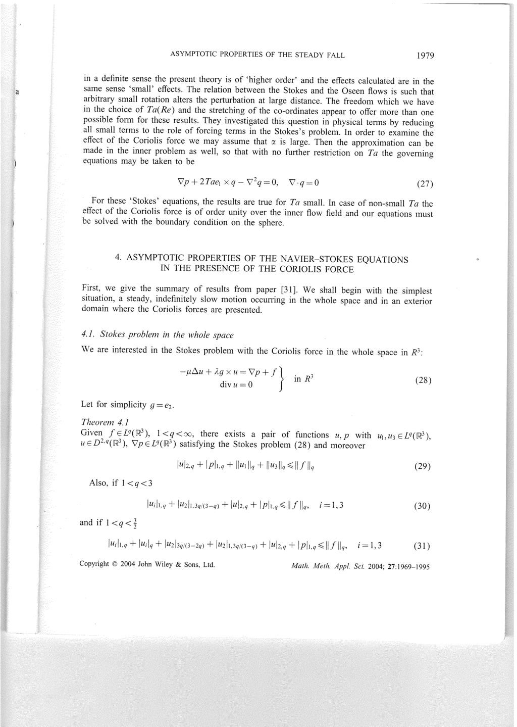
157

158

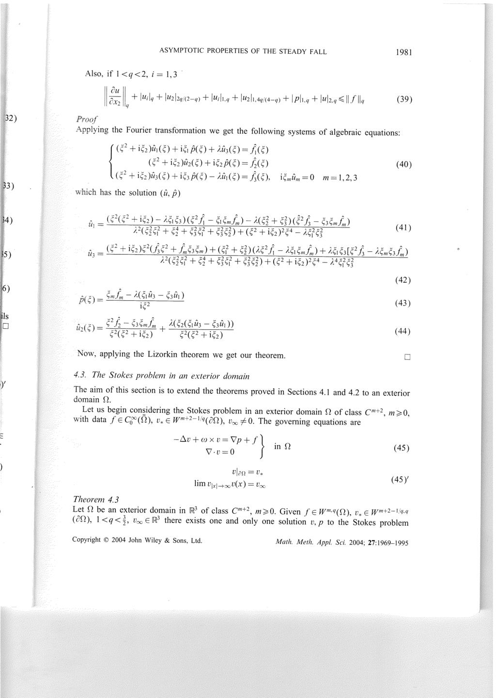
159

160

161

162

163

164

165

166

167

168

169

170

171

172

173

174

175

176

177

178

179

180

181

182

183

184

185

186

187

188

189

190

191

192

193

194

195

196

197

198

199

200

201

202

203

204

205

206

207

208

209

210

211

212

213

214

215

216

217

218

219

220 Nonlinear Analysis 72 21) Contents lists available at ScienceDirect Nonlinear Analysis journal homepage: Global existence of solutions for the one-dimensional motions of a compressible viscous gas with radiation: An infrarelativistic model Bernard Ducomet a, Šárka Nečasová b, a CEA, DAM, DIF, F Arpajon, France b Mathematical Institute AS ČR Žitna 25, Praha 1, Czech Republic a r t i c l e i n f o a b s t r a c t Article history: Received 23 October 29 Accepted 2 December 29 MSC: 35Q3 76N1 We consider an initial boundary value problem for the equations of 1D motions of a compressible viscous heat-conducting gas coupled with radiation through a radiative transfer equation. Assuming suitable hypotheses on the transport coefficients, we prove that the problem admits a unique weak solution. 29 Elsevier Ltd. All rights reserved. Keywords: Compressible Viscous Heat-conducting fluids One-dimensional symmetry Radiative transfer 1. Introduction The aim of radiation hydrodynamics is to include the effects of radiation into the hydrodynamical framework. When equilibrium holds between the matter and the radiation, a simple way to do that is to include local radiative terms into the state functions and the transport coefficients. One knows from quantum mechanics that radiation is described by its quanta, the photons, which are massless particles traveling at the speed c of light, characterized by their frequency ν, Ω, where Ω is a unit vector. Statistical mechanics allows us to describe macroscopically an assembly of massless photons of energy E and momentum p by using a distribution function: the radiative intensity Ir, t, Ω, ν). Using this fundamental quantity, one can derive global quantities by integrating with respect to the angular and frequency variables: the spectral radiative energy density E R r, t) per unit their energy E = hν where h is Planck s constant), and their momentum p = hν c volume is then E R r, t) := 1 c Ir, t, Ω, ν) dω dν, and the spectral radiative flux FR r, t) = Ω Ir, t, Ω, ν) dω dν. If matter is in thermodynamic equilibrium at constant temperature T and if radiation is also in thermodynamic equilibrium with matter, its temperature is also T and statistical mechanics tells us that the distribution function for photons is given by the Bose Einstein statistics with zero chemical potential. In the absence of radiation, one knows that the complete hydrodynamical system is derived from the standard conservation laws of mass, momentum and energy by using Boltzmann s equation satisfied by the f m r, v, t) and the Corresponding author. Tel.: addresses: bernard.ducomet@cea.fr B. Ducomet), matus@math.cas.cz Š. Nečasová) X/$ see front matter 29 Elsevier Ltd. All rights reserved. doi:1.116/j.na