NAVIGATION ALGORITHM FOR INS/GPS DATA FUSION

Transkript

1 VYSOKÉ UČENÍ TECHNICKÉ V BRNĚ BRNO UNIVERSITY OF TECHNOLOGY FAKULTA STROJNÍHO INŽENÝRSTVÍ LETECKÝ ÚSTAV FACULTY OF MECHANICAL ENGINEERING INSTITUTE OF AEROSPACE ENGINEERING NAVIGATION ALGORITHM FOR INS/GPS DATA FUSION NÁVRH ALGORITMU PRO FÚZI DAT NAVIGAČNÍCH SYSTÉMŮ GPS A INS DIPLOMOVÁ PRÁCE MASTER'S THESIS AUTOR PRÁCE AUTHOR VEDOUCÍ PRÁCE SUPERVISOR Bc. MARKÉTA PÁLENSKÁ doc. Ing. JAN ČIŽMÁR, CSc. BRNO 2013

2

3

4 Abstrakt Diplomová práce se zabývá návrhem algoritmu rozšířeného Kalmanova filtru, který integruje data z inerciálního navigačního systému (INS) a globálního polohovacího systému (GPS). Součástí algoritmu je i samotná mechanizace INS, určující na základě dat z akcelerometrů a gyroskopů údaje o rychlosti, zeměpisné pozici a polohových úhlech letadla. Vzhledem k rychlému nárůstu chybovosti INS je výstup korigován hodnotami rychlosti a pozice získané z GPS. Výsledný algoritmus je implementován v prostředí Simulink. Součástí práce je odvození jednotlivých stavových matic rozšířeného Kalmanova filtru. Summary This diploma thesis deals with Extended Kalman Filter algorithm fusing data from i- nertial navigation system (INS) and Global Positioning System (GPS). The part of the developed algorithm is a mechanization of INS which processes data from accelerometers and gyroscopes to provide velocity, position and attitude angles. Due to rapid increase of INS output errors, the EKF is used to correct INS outputs by velocity and position from GPS. The final algorithm is developed in Simulink environment. This thesis includes derivation of EKF state matrices. i

5 Klíčová slova Rozšířený Kalmanův filtr, inerciální navigační systém, integrace INS/GPS, algoritmus pro fúzi dat Key words Extended Kalman Filter, inertial navigation system, INS/GPS integration algorithm, sensor data fusion Bibliographic citation PÁLENSKÁ, M. Navigation algorithm for INS/GPS data fusion. Brno: Vysoké učení technické v Brně, Fakulta strojního inženýrství, s. Vedoucí diplomové práce doc. Ing. Jan Čižmár, CSc. ii

6 Declaration I declare that I have written the master s thesis Navigation algorithm for INS/GPS data fusion on my own according to the instructions of my master s thesis supervisor doc. Ing. Jan Čižmár, CSc., and using the sources listed in the references. May 20, 2013 Markéta Pálenská iii

7 I would like to thank my supervisor doc. Ing. Jan Čižmár, CSc. for presiding over my master s thesis. Many thanks belong to my consultants from Honeywell, Ing. Marek Fojtách and Ing. Jan Tomáš, Ph.D. for their support and provided knowledge. iv

8 Contents 1 Introduction Outline of thesis Current status of solved problematics Inertial Navigation Systems Coordinate frames Earth-Centered Inertial Frame Earth-Centered Earth-Fixed Frame Local Navigation Frame Wander Azimuth Frame Body Frame Transformation Equations Quaternion Direction Cosine Matrix Euler Angles Rotation Vector INS Mechanization Velocity Update Position Update Attitude Update Gravity Vector Update Inertial Sensors Error Model Biases Scale Factor and Cross-Coupling Errors Random noise Alignment of INS INS/GPS Data Fusion Global Positioning System GPS signal and its processing v

9 3.2 Integration Schemas Loosely Coupled Integration Tightly Coupled Integration Deep integration Kalman Filtering Extended Kalman Filter Development of integration algorithm Attitude Error Analysis Velocity Error Analysis Position Error Analysis Applying corrections Achieved Results Simulink model description Results Conclusion Summary Future work recommendations Conclusion vi

10 List of Figures 2.1 Attitude angles [2] ECI frame [5] ECEF frame [5] N-frame [5] B-frame [3] Schematic of an inertial navigation processor [1] The scale factor error [2] Open and closed loop of INS/GPS data fusion [1] Loosely coupled integration [1] Tightly coupled integration [1] Deep integration [1] Kalman filter algorithm steps [1] Operation of EKF [15] Schematic of my INS solution Schematic of my EKF architecture True values of position True values of velocity True values of attitude Position errors from INS with ideal sensors Velocity errors from INS with ideal sensors Attitude errors from INS with ideal sensors Position errors from INS with noisy accelerometers Velocity errors from INS with noisy accelerometers Position errors from INS with noisy sensors Velocity errors from INS with noisy sensors Attitude errors from noisy sensors GPS Position errors GPS Velocity errors Simple EKF Position errors (noise only in accelerometers) vii

11 5.17 Simple EKF Velocity errors (noise only in accelerometers) Full EKF Position errors Full EKF Velocity errors Full EKF Attitude errors The Allan Variance on ifog-imu-1-a for accelerometer and gyroscope in x-axis viii

12 List of Symbols δ 1 T Time derivative Error of Inverse matrix Transposed matrix Cross product ( ) Skew symmetric form of a vector E( ) ( ) A b C b a C(t) D(t) ε e f f F θ ϕ Expectation of Summation Coriolis force Bias vector Direction cosine matrix C/A code GPS Navigation message Attitude error vector First eccentricity of ellipsoid Flattening of the ellipsoid Specific force vector State transition matrix Pitch angle Geodetic Latitude ix

13 Φ g H h I K λ ρ φ ω Ω P q Q r R 0 R N R M R T u x y Transition matrix Gravity vector Measurement matrix Geodetic altitude Identity matrix Kalman gain Geodetic longitude Rotation vector Roll angle Angular rate vector Skew-symmetric matrix of angular rate vector Covariance matrix of state vector Quaternion Covariance matrix of system noise vector Position vector Equatorial Earth radius Prime vertical radius of curvature Meridian radius of curvature Covariance matrix of measurement vector Sample time Output vector of IMU State vector Measurement vector x

14 Chapter 1 Introduction There are two possible approaches to navigation. The first is position fixing method based on measuring the ranges and bearings to known objects [1]. The Global Positioning System is an example of position fixing method. The second way called dead reckoning method which is based on measuring the changes in navigation quantities. These changes are integrated and added to previous values to get the actual value. These two approaches exibit complementary positives and negatives. Thus, integrated navigation solution provides benefits of both methods. Inertial navigation systems are among navigation systems based on dead reckoning. The INS has an impressively simple physical background. Fundamental idea comes from Newton s second motion of law and basic kinematics. Newton s second motion of law says that sum of forces acting the body is directly proportional to the mass and acceleration of the body. When acceleration of the body is measured with knowledge of initial conditons there can be simply found immediate velocity and position by integrating this with respect to time. This implies the important advantage of these systems which is autonomy - inertial navigation systems do not need any external equipment except sensors (accelerometres and gyroscopes sensing the accelerations and angular rates) and navigation processor providing navigation solution. Thus, they are independent of external electromagnetic signals. Next advantages of INS are high short-term accuracy and short period output rate [1]. The continuous operation provides not just velocity and position, but also attitude 1, angular rates and accelerations. Disadvantages include rapid increase of error with time due to integration in the calculation. Outputs from accelerometres and gyroscopes are corrupted by noises and biases and without corrections result in unbounded errors. This is more noticeable in case of low-cost sensors as sensors based on MEMS technology. High performance sensors used e.g. in military and spacecraft application provide more precision but costs are about hundred thousands dollars [1]. 1 When magnetometres are not part of sensors, the precision in heading is not sufficient 1

15 Global Positioning System as a system using position fixing method offers complementary positives and negatives. Low cost of user equipment and high long-term accuracy belong among the advantages of GPS. On the contrary this system is characterized by long period of output rate and possible unavailability because GPS is vulnerable to interference. Also high bandwidth noise is characteristic for GPS. Next potential drawback is a high short-term noise. Complete navigation system fusing both of them results in high performance and robustness due to complementary attributes of INS and GPS. A typical integration architecture means that measurements from GPS used by an estimation algorithm to apply corrections to the navigation solution of INS. Estimation theory provides a powerful tool to estimate states of interest in aided navigation system. This tool is Kalman filter and it is a key to get an optimal solution from both measurements. Although the name, Kalman filter is an estimation algorithm, rather then a filter [1]. It was invented in 1960s by a Hungarian mathematician R.E.Kalman [8]. This tool applies to wide range of disciplines but has irreplaceable function in control systems, avionics and space applications. The first aim of the thesis is to create mechanization of inertial navigation system. Inputs to the system are data from three accelerometres and three gyroscopes and outputs are immediate values of attitude (roll, pitch and yaw angle), velocity and position. Model of INS is created in Simulink environment and sources of data are supplied by company Honeywell International s.r.o. The second step is to implement an Extended Kalman Filter to apply corrections based on GPS measurements to outputs of INS. Thus, the final algorithm should be INS aided by GPS. The assigned task is to create an error state model of EKF which estimates values of corrections to attitude, velocity and position and further noise parametres of sensors to correct sensor outputs directly. The aim of the work is a system corrected as at the input (removing computed biases in every step) and as at the output (corrections to computed navigation quantities in every step). 1.1 Outline of thesis This diploma thesis contains six chapters. Chapter 1 focuses on the basic summary of the thesis with emphasis on the current status of the INS/GPS fusion common approach. Chapter 2 describes the overview of INS, focused on the mathematical equations describing the implemented INS mechanization. The chosen approach to the creation of functional model of INS is presented and the necessary theory concerning the reference frames and transformation of the quantities between them. The term of INS mechanization is understood as a set of equations giving a solution in the form of position, velocity and attitude from inputs to the system (measured accelerations and angular rates). 2

16 At the beginning of Chapter 3, different integration schemas of INS and GPS are studied with their pros and cons. Thus, the selected algorithm of data fusion - Extended Kalman filter (EKF) is presented. In Chapter 4 single matrices necessary to create an EKF algorithm are derived and some implementation issues are discussed. The Chapter 5 presents achieved results and describes developed Simulink models. The Chapter 6 summarizes the thesis and provides suggestions for next work. Appendixes to thesis present discretization of INS velocity equation and practical use of Allan Variance (method suitable for analyzing inertial sensors). 1.2 Current status of solved problematics Kalman filter as an extremely powerful tool for analyzing estimation problems was developed in 1960s. The next step was the development of the MEMS technology in 1970s and their progress in the next decades enabling the quartz and silicon sensors to be mass produced at low cost using etching techniques with several sensors on a single silicon wafer [1]. The MEMS sensors are small and light, but currently their performance is relatively low. These lower grade inertial sensors are not suitable for inertial navigation, but their performance can be rapidly increased by integrating with a different navigation system (often GPS). Then even using these sensors in aerospace industry (rather in AHRS 2 than in INS) is possible. The connection of one of the great breakthroughs in estimation theory, Kalman filter, with MEMS technology significantly expands possibilities in use of inertial sensors. My work is focused on Extended Kalman Filter algorithm to fuse data from INS and GPS. Nowadays some advanced INS/GPS integrations schemes exist. For example differential GPS improves position accuracy by calibrating out much of the temporally and spatially correlated biases in the pseudo-range values due to ephemeris prediction errors and residual satellite clock errors, ionospheric refraction or even tropospheric refraction [1]. The next possibility to increase performance of the MEMS sensors is the use of the adaptive Kalman filter to vary the assumed system noise. This approach results in speeding up the time of convergence of the state estimates with their true counterparts [1]. While Kalman filter is an ideal solution for real-time application, Kalman smoother is the way in such a case when measurements are needed after as well as before the time of interest. Kalman smoothing is realized by two main methods - the forwardbackward method and Rauch, Tung and Striebel method. More detailed information and next extensions to Kalman Filter can be found e.g. in [1]. Recommended and actual sources to get detailed information about the topic discussed in this thesis are mainly [1], [2] and [5]. 2 Attitude and Heading Reference System 3

17 Chapter 2 Inertial Navigation Systems Inertial Navigation System contains Inertial Measurement Unit, which is a set of three mutually orthogonal accelerometres and three gyroscopes measuring angular rates. Outputs from accelerometres are processed to get position and velocity, angular rates are processed to get attitude. Thus, outputs from INS are following: vel = [v N v E v D ] T pos = [ϕ λ h] T att = [φ θ ψ] T (2.1) where attitude angles (roll, pitch and yaw angle) describing rotation about axes of aircraft. The aeronautical convention defining these parametres as shown at Figure 2.1. Figure 2.1: Attitude angles [2] 4

18 Values measured by accelerometres are called specific forces. Specific force is the acceleration due to all forces except gravity [1]. An important conclusion is that the acceleration does not equal to specific force except situation with zero tilt angle. This is one reason to know attitude to compensate it. There are two commonly used mechanizations: Strapdown or gimbaless INS means that sensors are strapped into vehicle and are aligned with the navigation body. Therefore, the sensors rotate with vehicle. The alignment is done in navigation processor analytically. Strapdown INS has much simple mechanical construction but exhibits higher error rates due to sensor movement in all directions and following gravity influencing of all sensors. Stabilized mechanization means that the instrument platform is isolated not to rotate with vehicle. The angle to the gravity vector is constant. Transformation of the measured values from body to navigation frame is not needed. Due to smaller dynamic range, the sensing provides higher accuracy [5]. Gimbals arrangement can be very complicated and with high maintenance costs. When need of change some sensor occurs, complicated system must be dismantled and then completed in surgically clean environment, not to mention long calibration procedures [6]. Further strapdown INS will be considered. 2.1 Coordinate frames Transformation of measured and computed quantities between various reference frames is needed. User wants to get his position in geographic coordinates. Sensor outputs are relative to inertial frame of reference, but the rotating Earth does not satisfy conditions of inertial frame. GPS also determines the position of receiver with a respect to satellites. Reference frames and transformation procedure are described in this chapter Earth-Centered Inertial Frame Newton s laws are valid only in inertial frame of reference. Inertial frame of reference means non-rotating and non-accelerating frame. Earth-Centered Inertial Frame has a center at the Earth s center of gravity. Axes are non-rotating and directed to the distant stars. Z-axis is parallel to the spin axis of the Earth, x-axis points to the vernal equinox point ant the y-axis is the axis completing right-handed orthogonal frame. The vernal equinox is the point of intersection of ascending node of ecliptic and the celestial equator. 1 ECI frame is marked by a notation i. 1 This reference frame also doesn t satisfy conditions for inertial frame due to non-constant velocity of Earth s motion around the Sun and due to Galaxy s rotation. This approximation is sufficient for navigation purposes. 5

19 Figure 2.2: ECI frame [5] Figure 2.3: ECEF frame [5] Earth-Centered Earth-Fixed Frame The origin of the ECEF frame is at the Earth s center of gravity. Axes are fixed with respect to the Earth. Z-axis is the same as at the i-frame, x-axis points to mean meridian of Greenwich and y-axis completes right-handed orthogonal frame. The rotation rate vector of the e-frame with respect to the i-frame projected in e-frame is defined as [3]: ω e ie = [0 0 ω ie ] T (2.2) The angular velocity of e-frame relative to i-frame is ω ie = 7, rad s -1 according to WGS 84. The constant rotation rate is assumed for navigation purposes although sidereal day 2 has not constant length. Variations are caused by wind, ice forming and melting and their size do not exceed several milliseconds [5]. ECEF frame is marked by a notation e. Position vector in the e-frame is computed according to the equation 2.3 [3]: x r e = y = z (R N + h)cosϕ cosλ (R N + h)cosϕ sinλ (R N (1 e 2 ) + h)sinϕ (2.3) where ϕ means geodetic latitude, λ denotes geodetic longitude, h altitude, R N is the radius of curvature in the prime vertical and e is the first eccentricity of the reference 2 Sidereal day is the period of rotation of the Earth with respect to the distant stars, solar day is defined with respect to the Sun 6

20 Figure 2.4: N-frame [5] ellipsoid Local Navigation Frame The origin of local navigation frame is at the point of the initial location of sensors. This frame is crucial for user because there is a need to know a position relative to north, east an down directions. Thus, this frame is also called as a NED coordinate system. X-axis points to the true north, z-axis is orthogonal to the surface of the reference ellipsoid and y-axis points to the east and completes the right-handed orthogonal frame. The notation of the local frame is n-frame. The use of n-frame causes problems around the Earth s poles. To maintain orientation of x-axis to the north, the rotation about z-axis occurs. When strapdown system is used, rotation is performed just analytically, but problem appears when the stabilised platform is used. The solution is the use of w-frame Wander Azimuth Frame The distinction between n-frame and w-frame is in the shift of x and y-axes. The angle of displacement is called a wander angle. The wander angle is equal to the meridian convergence from the point of alignment [7]. Using w-frame instead of n-frame avoids problems with singularity around Earth s poles Body Frame The body frame or also vehicle frame is tightly bounded to the platform where sensors are placed. Its origin is identical with the origin of the local navigation frame, but the axes are aligned with the movement of vehicle. Outputs from accelerometres and gyroscopes are measured in the body frame and then are transformed. The x-axis of the body frame corresponds to roll axis, y-axis corresponds to pitch axis and z-axis corresponds to yaw axis. 7

21 Figure 2.5: B-frame [3] 2.2 Transformation Equations Approaches to transform quantities from one coordinate frame to another are described in this section. Commonly used techniques are quaternions, Euler angles, direction cosine matrixes and rotation vectors. Detailed description can be found e.g. in [1]. Imaginary frames a and b are used to describe each method of transformation Quaternion Quaternion is described as a non-commutative extension of complex numbers with the scalar part and three dimensional vector part. The scalar part s = q 0 represents the magnitude of rotation and the vector part v = [q 1 q 2 q 3 ] represents the axis about which that rotation takes place [1]. The main advantage is that quaternions do not suffer from gimbal lock. The next advantage is an amount and linearity of equations, on the other hand this approach is not too intuitive. The quaternion attitude definition: [ ] s q = = v q 0 q 1 q 2 q 3 = cos( µ 2 ) u 1 sin( µ 2 ) u 2 sin( µ 2 ) u 3 sin( µ 2 ) (2.4) where µ represents the rotation angle and u = [u 1 u 2 u 3 ] is the unit vector describing rotation axis. Definition of product of two quaternions [3]: [ ] q a b = qa c q c b = s 1 s 2 v T 1 v 2 (2.5) s 1 v 2 +s 2 v 1 + v 1 v 2 Quaternion obtained from DCM [1]: q 0 = c11 + c 22 + c 33 8

22 q 1 = c 32 c 23 4q 0 q 2 = c 13 c 31 4q 0 q 3 = c 21 c 12 4q 0 (2.6) Quaternion obtained from Euler angles [3]: cos φ 2 cos ψ 2 cos θ 2 + sin φ 2 sin ψ 2 cos θ 2 q = sin φ 2 cos ψ 2 cos θ 2 cos φ 2 sin ψ 2 sin θ 2 cos φ 2 sin ψ 2 cos θ 2 + sin φ 2 cos ψ 2 cos θ 2 cos φ 2 cos ψ 2 sin θ 2 sin φ 2 sin ψ 2 cos θ 2 (2.7) Quaternion obtained from rotation vector [3]: cos 0.5ρ q= sin 0.5ρ 0.5ρ 0.5ρ (2.8) where cos 0.5ρ =1 0.5ρ 2 2! + 0.5ρ 4 4!... sin 0.5ρ = 1 0.5ρ 2 3! Symbol means Euclidean form ρ 4 5! Direction Cosine Matrix Direction Cosine Matrix (DCM) is the matrix of size 3 3. Ca b means DCM transforming vector from coordinate frame a to coordinate frame b. When using DCM, differential equations are linear and no singularity can occur, but the number of equations which needs to be considered is higher than other approaches. DCM expressed using rotation vector [3]: C b a = I + sin ρ ρ 1 cos ρ (ρ ) + ρ 2 (ρ )(ρ ), (2.9) where symbol ρ denotes skew-symmetric matrix 3 of vector ρ = [ρ x ρ y ρ z ]: 3 Skew-symmetric matrices are used to avoid vector multiplication 9

23 (ρ ) = 0 ρ z ρ y ρ z 0 ρ x ρ y ρ x 0 (2.10) DCM obtained from quaternions [1]: q 2 0 Ca b + q2 1 q2 2 q2 3 2(q 1 q 2 q 3 q 0 ) 2(q 1 q 3 + q 2 q 0 ) = 2(q 1 q 2 + q 3 q 0 ) q 2 0 q2 1 + q2 2 q2 3 2(q 2 q 3 q 1 q 0 ) (2.11) 2(q 1 q 3 q 2 q 0 ) 2(q 2 q 3 + q 1 q 0 ) q 2 0 q2 1 q2 2 + q2 3 DCM obtained from Euler angles [1]: cosθ cosψ ( cosφ sinψ + sinφ sinθ cosψ) (sinφ sinψ + cosφ sinθ cosψ) Ca b = cosθ sinψ (cosφ cosψ + sinφ sinθ sinψ) ( sinφ cosψ + cosφ sinθ sinψ) sinθ sinφ cosθ cosφ cosθ Euler Angles (2.12) Euler angles are a very intuitive kind of representation attitude. This trinity of angles [θ φ ψ] describes rotation around three axes x, y and z. In such a case when the attitude of the body frame with respect to the local navigation frame is described, the roll rotation φ represents bank, the pitch rotation θ is elevation and ψ is known as heading. Disadvantage of this method is non-linearity of equations and singularity at ±90 degrees. Euler Angles obtained from DCM [3]: θ = tan 1 c 31 c c2 33 (2.13) φ = tan 1 c 32 c 33 (2.14) ψ = tan 1 c 21 c 11 (2.15) Euler Angles computed from quaternion [1]: θ = tan 1 2(q 0q 1 + q 2 q 3 ) 1 2(q 2 1 q2 2 ) (2.16) φ = sin 1 (2(q 2 q 0 q 1 q 3 )) (2.17) 10

24 ψ = tan 1 2(q 0q 3 + q 1 q 2 ) 1 2(q 2 2 q2 3 ) (2.18) Rotation Vector Describing rotation by rotation vector is a method coming from Euler s and Chasles s theorems. Information about vector which rotation occurs around and rate of rotation is needed for describing an attitude relative to local navigation frame [8]. The positive features of this method include the fact that differential equations explicitly account for non-commutavity effects. Among the disadvantages are the non-linearity of equations and singularity at 2nπ rad. When small angle approximation is used, the rotation vector coincides with Euler angles. Rotation vector obtained from quaternion [3]: ρ = 1 k [q 1 q 2 q 3 ] T (2.19) k = 1 0,5ρ 2 (1 + 0,5ρ 4 0,5ρ ) (2.20) 2 3! 5! 7! 0,5ρ = q q2 2 + q2 3 q 0 (2.21) Rotation vector obtained from DCM [3]: ρ= χ c 23 c 32 c 2sin χ 31 c 13 (2.22) c 12 c 21 where [ ] tr(c b χ= arccos a ) 1 2 where tr(c b a) denotes trace of matrix. 2.3 INS Mechanization Mechanization of INS is a process where outputs from accelerometres and gyroscopes are used to obtain navigation solution - values of attitude, velocity and position in n- frame. There is a consensus at continuous time equations as a result of more than twenty years of strapdown INS development [3]: v n =C n b f b + g n (2ω n ie + ω n en) v n (2.23) 11

25 Figure 2.6: Schematic of an inertial navigation processor [1] C e n=c e n(ω n en ) (2.24) ḣ= v D (2.25) Ċb n = Cn b (ωb ib ) (ωn in )Cb n (2.26) where Cb n means direction cosine matrix from b-frame to n-frame and gn is a vector of gravity. The angular rates have following meaning: ωie n is Earth s rotation rate with respect to i-frame and ωen n means turn rate of the n-frame with respect to the e-frame. Cn e is a Direction Cosine Matrix from n-frame to e-frame and v D is a downward velocity. Angular rate ωib b is measured by IMU and ωn in is computed as a sum of ωn ie and ωn en. Implemented equations are given by discretizing these equations. Common process of computing navigation quantities is described at Figure 2.6. The model is realized in the Simulink environment and works on frequency 100 Hz. Subsystem Trajectory Generator was supplied by Honeywell International company. It contains following data: IMU sensor outputs and true values about position, velocity and attitude used for verification of the correct function Velocity Update Velocity in n-frame is calculated using equation This equation is in continuous form. Laplace transform and Z-transform was applied to get this equation in discrete form. The process of derivation is provided in Appendix A. After discretization, the implemented equation is as follows: 12

26 [( v n k = (I + AT 2 ) 1 I A T ) v n k T ] 2 (Cn b(k) F k +Cb(k 1) n F k 1 + G k + G k 1 ) (2.27) Symbols k and k 1 mean current and previous state. T is a sample time and I is an unit matrix of size 3 3. Matrix A is given by the equation 2.28 and represents Coriolis force correction. The actual value of Coriolis force correction is a sum of doubled Earth rate and transport rate. This sum is transformed from vector to skew-symmetric matrix. A = (2ω n ie + ω n en) (2.28) Position Update Equations in continuous form [8]: v n ϕ= R M + h (2.29) λ = v E (R N + h)cosϕ Derivation of altitude h is computed according to equation Thus, implemented equations are following: ˆ λ= ˆ ϕ= (2.30) v n R M + h dv N (2.31) v E (R N + h)cosϕ dv E (2.32) ˆ h = v D dv D (2.33) Attitude Update There is a need to say that results in yaw angle exhibit more inaccuracy than in the roll and pitch angle. The justification is that for complex AHRS solution magnetometres are next necessary sensors to precise heading computation. Thus, greater inaccuracy in the yaw angle is not caused by an error in algorithm. Attitude is computed using equation Implementation was obtained from [5]: [ q k = cos ν 2 I + 2 ] ν sin ν 2 Ω q k 1 (2.34) q is a symbol of quaternion, ν and Ω are quantities computed according to [5]: 13

27 Constant name Value Earth s gravitational constant µ = m 3 s 2 Earth s angular rate ω ie = rads 1 1 Flattening of the ellipsoid f = Eccentricity of the ellipsoid e= Equatorial radius R 0 = m Polar radius R P = m Table 2.1: WGS 84 values used for the computing of the gravity vector ν= ω n bn = {[ω b ib(k 1) Cb n(k 1) ωn in ] [ ]} T + ωib(k) b Cb n(k) ωn in 2 (2.35) 0 ν x ν y ν z Ω = ν x 0 ν z ν y ν y ν z 0 ν x ν z ν y ν x 0 (2.36) Thus DCM is obtained from quaternion using 2.11 and Euler angles are obtained from DCM usinq equations 2.13 to Matrix Ω is called as a skew-symmetric matrix of vector ν Gravity Vector Update Gravity vector is computed from actual position according to the following equations [1]: [ g = g(ϕ) 1 2 (1 + f + ω2 ie R2 0 R P )h + 3 ] R 0 µ R 2 h 2 0 (2.37) g(ϕ) = sin2 ϕ 1 e 2 sin 2 ϕ (2.38) The equation 2.38 describes a simple WGS-84 model of the acceleration due to gravity at the ellipsoid as a function of latitude. This is a gravity field model including outward centrifugal acceleration due to Earth s rotation (virtual force arising from the use of rotating resolving axes). To get rid of this acceleration and obtain just gravitational acceleration there is a need to subtract this. Thus, gravitational acceleration varies with height and needs to be scaled. This resulted in equation 2.37 [1]. Used values of Earth s parameters are taken from WGS 84 and are summarized in Table The direct conversion from quaternion to Euler angles is not used, because direction cosine matrix is used for the computing of velocity 14

28 2.4 Inertial Sensors Error Model Inertial sensors are accelerometres and gyroscopes measuring specific forces and angular rates without external device. There are various types of inertial sensors. Accelerometres can operate on the piezoelectric or capatitive principle to convert mechanical motion into an electrical signal. Technology of gyroscope can be fiber-optical, ring laser or based on spinning mass [1]. Used technology differs in cost, size, performance, possible use and other factors. The current status of the development of low-cost sensors is marked by using MEMS technology. MEMS (Micro-Electrical-Mechanical Systems) technology uses sophisticated placement of electronical and micro-mechanical elements to silicon wafer via etching technology. The advantages of MEMS sensor are small size and weight, low cost and power consumption and relatively great shock tolerance. Of course, their performance is poor in comparison to very accurate laser-ring sensors. There is no perfect sensor without any error. Every sensor output is corrupted and there is a need to analyze errors and remove the maximum possible amount of thems. The errors of IMU sensors can be divided into several categories. They include biases, scale factor, cross-coupling errors and random noise Biases The bias is a constant error exhibited by all accelerometers and gyros. The bias is often one of major contributors to overall error. Bias is the composition of static and dynamic part. The static component of bias (also known as bias offset) is constant through IMU operation, but it differs run-to-run [1]. Bias offset can be calibrated by measurement without any IMU input. The dynamic part is called bias instability or inrun bias variation and varies over period of order a minute. Typically it represents about 10 % size of the static bias [1]. Accelerometer bias is denoted as b a = (b a,x,b a,y,b a,z ) and respectively gyro bias is denoted as b g = (b g,x,b g,y,b g,z ) Scale Factor and Cross-Coupling Errors The scale factor error represents error in the mapping of the input-output relationship. The scale factor error of sensor output is proportional to the true value. The denoting of accelerometer scale factor errors is s a = (s a,x,s a,y,s a,z ) and the denoting of gyroscope scale factor error is s g = (s g,x,s g,y,s g,z ). The scale factor is illustrated at Figure 2.7. Cross-coupling error (or misalingnment error) comes from misalingnment of the sensitive axes. It is caused by production constraints. Generally, misalingnment errors do not significinantly contribute to overall error, even though some low-cost IMU sensors can be exception. 15

29 Figure 2.7: The scale factor error [2] Random noise Random noise occurs in all IMU sensors and it is caused by various reasons. Mechanical instabilities are manifested at spinning-mass gyros, high-frequency resonances cause noise in vibratory gyros etc. MEMS sensors are loaded with a lot of random noise. The denotation is w a = (w a,x,w a,y,w a,z ) at accelerometres and w g = (w g,x,w g,y,w g,z ) at gyroscopes Alignment of INS IMU sensor outputs are integrated to get the navigational solution. This implies the need of the initial estimation of values. The estimation includes initialization, calibration and alignment. The initial phase of ground alingnment is the levelling which provides the estimate of initial attitude. The alignment is defined as determining the relative orientation of the INS platform and the reference navigation frame axes. The initialization means initial estimate of velocity and position and calibration is a process of determining of various factors to calibrate inertial instruments [2]. The calibration of IMU sensors can be off-line in laboratory or on-line using stateaugmentation techniques. The initial estimate of velocity, position and attitude with their error is needed at least at the start of operating. When aiding INS is considered, estimates are further needed. Correct initialization is important not just to get integrating constants. For example, the incorrect estimate of position affects gravity vector and Coriolis force compensation. Also wrong estimate of initial attitude results in incorrect velocity computation etc. Thus, alignment, initialization and calibration are critical to system performance [2]. The problem of initialization is often solved via estimation theory. Therefore, the initialization is performed using the same tools as normal operation (when aided INS is used). 16

30 Chapter 3 INS/GPS Data Fusion Brief reasons to integrate INS and GPS were presented in Chapter 1. Complementary disadvantages of these systems exhort to use both of them together. The dominant errors of INS are low frequency drifts, on the contrary the main GPS error consists in high bandwidth noise. But there are other possible navigation systems which can be used to aid INS. In the area of personal navigation, odometres or some other low-cost dead-reckoning systems are used [1]. In aviation, the fusion of INS and GPS is an ideal solution to get continuous high bandwidth information. Due to the development of MEMS technology, the price of inertial sensors has been significantly decreased. The weaknesses of GPS include the vulnerability to outages, low data rate and no attitude information 1. On the other hand, the GPS errors are bounded and the GPS equipment is cheap. INS is an autonomous system with high data rate, but is susceptible to error drifting. Any inaccuracy in sensor informations due to integration in INS mechanization leads to errors which grow with time. Prices of IMUs which provide sufficient-quality solutions for periods longer than the order of minutes are very high. So, integration of GPS and INS allows to create a reliable navigational system even with inexpensive inertial sensors. There exists several integration approaches. They differ in a way how corrections gained from integration algorithm are applied back to the INS, what types of GPS information are used (if just position and velocity or directly pseudorange and carrier phase) and if GPS equipment uses outputs from integration algorithm or not. Integration algorithm can work as the total state or as the error state - in the first case the algorithm computes true values of navigational quantities, in the case of error state approach the algorithm computes corrections (distinctions from true values are intended). As the assignment of my thesis is the error state approach, only this method will be discussed further. There is no precise definition of particular integration approaches, so commonly 1 If carrier phases with multiple antennas are not used [8]. 17

31 Figure 3.1: Open and closed loop of INS/GPS data fusion [1] used terms according to Groves are presented. Basic types are loose, tight and deep integration differing in the degree of integration. The greater degree of integration brings better performance and higher reliability, but on the other hand the independence of both systems is lost. My thesis focuses on the loose integration, thus this type is described more detailed. The integration schemas can also be divided into open or closed solutions. In other words, if computed corrections of sensors are fed back to the INS (closed loop) or if just corrections to INS outputs are processed (open loop). Decision about suitable approach is a question of quality of inertial sensors and integration algorithm. Higher quality sensors with not so powerful algorithm justifies use of open loop. When ratio of quality is opposite, the use of closed loop makes more sense. The issue is if raw data from sensors are meaningful to maintain and use the open-loop configuration as integrity monitoring. Based on quality of analyzed and simulated sensors, the closed loop solution was chosen. 3.1 Global Positioning System GPS is the global navigation satellite system operated by U.S. Department of Defense. The GPS user equipment measures time delays and decodes messages from visible satellites to determine position and accurate time anywhere on Earth. Limited accuracy services are freely available to civil users. This section describes the basic principle of operating and typical error sources. GPS consists of three segments - space, control and user. The space segment contains from 24 to 32 satellites. Satellites move in six circular orbits at altitude of 20,200 km. These satellites broadcast signals to control segment and to users. The inclination angle relative to the equator is 55 degrees, the spacing of orbits is 60 degrees. The constellation is designed with at least four satellites visible anytime [9]. 18

32 The control segment represents the network of monitor stations which provides correction for each satellite. The next part of control segment are control stations which calculate the needed correction to the satellite motion 2 and the navigation data message to be send back to the space segment. The validity of each navigation message is several hours and contains data about ephemeris (precise satellite orbit), ionospheric refraction model etc. The user segment consists of passive users. Global Positioning Service provides two levels of accuracy - Precise Positioning Service (PPS) and Standard Precisioning Service (SPS). PPS is available just for authorized users (U.S. Army and selected allies armies). The approach to PPS is allowed by the decoding key. The PPS enables to achieve accuracy in tens of centimetres. SPS is a free service accesible to unlimited number of users with accuracy about 100 metres 3. The principle of GPS is based on time-of-arrival ranging [5]. The GPS receiver calculates the required time for transmission from the satellite to the receiver. This time interval is converted to distance by the multiplication by speed of light. This distance is called pseudorange due to errors in the satellite s and the receiver s clock. At least four satellites are needed for succesful positioning. One known range gives information that the searched position is on the sphere. Three ranges lead to the intersection of three spheres which gives two points. One of them can be excluded because approximate position is known. Thus, the fourth measure is needed for the elimination of the receiver clock s bias. Receiver clock s bias is time varying error that affects all simultaneous range measurements in the same manner [5]. This error can be estimated when four satellites are visible. The next type of error is a satellite clock s bias. This bias is estimated by monitor stations and then sent to the user segment to correct range. The atmospheric delay is an error caused by conditions influencing speed of light as temperature, pressure and humidity changes (tropospheric atmospheric delay) and level of air ionization (ionospheric atmospheric delay). Selective Availability errors are purposely added to decrease accuracy for nonauthorized users. The SA error can be achieved in two ways - by corrupting the broadcasting of ephemeris data or by dithering satellite oscillator frequency [5] GPS signal and its processing This subsection is based on [9]. Every GPS satellite broadcasts on two frequencies: L 1 = 1575,42 MHz 2 Maneuvres are known as station keeping used to keep correct satellite track. 3 Using differential GPS in the surroundings of control stations significantly improves accuracy. 19

33 L 2 = 1227,6 MHz The GPS signal is described by a following equation [9]: s(t) = A c C(t)D(t)sin(2ΠL 1 t) + A p1 P(t)D(t)cos(2ΠL 1 t) + A p2 P(t)D(t)cos(2ΠL 2 t) (3.1) Carrier waves are modulated by C(t) and D(t) codes. Codes and data have values +1 and 1. Thus, the modulation type is Binary-Phase Shift Keying (BPSK). The meaning of codes C(t) and D(t) is enabling of distance measuring and separation of individual satellite s signals. Data D(t) are used for ephemeris data transmission. Satellite positions are computed in user s receiver from ephemeris data. Codes are pseudorandom sequences used to increase resistence to interference (due to spread spectrum transmission). The next reason to use codes is for separation of satellites (code multiplex). Code C(t) is called Gold code. Gold codes have bounded small cross-correlations within a set, which is used for sharing frequency by multiple transmitters. The bit rate is 1,023 MB/s. The designation of this code is C/A, Coarse Acquisition. The code P(t) is so-called Precision code. It is a pseudorandom sequence with period of an aprrox. 266 days (but only seven days long part is used). The bit rate is 10,230 MB/s. This code enables greater precision due to longer and faster code which increases frequency spreading. Also user can measure at both frequencies when using P(t) code. Using of both frequencies helps to deal with ionospheric refraction. GPS errors is possible to divide into three groups. The first of them are errors formed in the space segment. These errors come mainly from stability of satellite s frequency issues and prediction of satellite s perturbance. Greater error obtained from the control segment comes from ephemeris prediction. At the side of user, the main part of error is ionospheric refraction. Further, the tropospheric refraction, receiver s noise or multipath propagation of signal contribute to overall error. 3.2 Integration Schemas Loosely Coupled Integration The loosely coupled integration of INS and GPS is characterized by the use of GPS outputs (position and velocity) to compare with INS output. Differences between INS and GPS solution are utilized as measurement. System model of estimation algorithm is based on INS error dynamics equations. The output from estimation algorithm, of- 20

34 Figure 3.2: Loosely coupled integration [1] ten the Extended Kalman Filter 4, is used as correction and applied back to the INS. The integrated navigation solution is then the corrected INS navigation solution. INS and GPS provide the independent solution and the estimation algorithm forms the third solution. The advantage is a simplicity, redundancy and existence of the independent GPS solution in case of the open-loop solution. Another advantage is the faster processing time (compared to the tightly coupled integration) due to smaller dimensions in state vectors [13]. When the loosely coupled integration scheme is selected, the important question is the choice of measurement iteration rate. Too rapid rate leads to instability, on the contrary too slow rate can cause less observability [1]. This method needs four visible satellites which limits the use for terrestrial applications. Also the situation with frequent outages of GPS requires more accurate sensors (to maintain acceptable precision during outages) Tightly Coupled Integration In case of tightly coupled integration input as measurement to the estimation algorithm are pseudo-range and pseudo-range rates from GPS [1]. The use of just one of them is possible, but in practice the use of both is advantageous due to their complementarity. 5 Satellite ephemeris data are used to derive pseudo-range from INS. The advantage of this way of integration is a greater resistance against interference and jamming and the fact that the integrated solution is avalaible even in such a case when less than four satellites are visible. The difficulty is that the system designer must have access to 4 Next possibilities are unscented Kalman filter or particle filters [12] 5 Pseudo-ranges come from code tracking and pseudo-range rates come from carrier tracking which is more accurate and less robust than code tracking [1]. 21

35 Figure 3.3: Tightly coupled integration [1] GPS equipment hardware. So this access is not suitable for general using [5]. Another disadvantage is the loss of independent GPS solution and greater computational load. According to Solimeno, the computational load (number of operations) of the tightly coupled system compared to the loosely coupled system increases linearly with the number of visible satellites Deep integration Deep integration approach (also known as ultra-tight) enables GPS outputs to be generated by means of the corrected INS solution, information from navigation data message and GPS error estimates. This architecture improves noise resistance. As well as the previous solution for short time intervals, this kind of system is operational when less than four satellites are available [1]. 3.3 Kalman Filtering The Kalman filter represents one of most widely used method to estimate variables in navigation systems. Its use enables to integrate measurements from various sources into optimal solution which provides better performance than either of them alone. This chapter presents basic principles of this algorithm. The Kalman filter is a linear statistical estimation algorithm invented by R. E. Kalman. The assumption is that the observed system is driven by noise which is characterized by stochastic quantities and that sensors are disrupted by the same type of noise. The Kalman filter is an optimal filter minimizing variance for known stochastic 22

36 Figure 3.4: Deep integration [1] linear model with gaussian zero-mean noise and known covariance [6]. The estimator is driven by same inputs as the observed system and the estimate is based on comparing both inputs (computed and measured). The algorithm estimates system parametres in real time based on measuring. Measurements are function of estimated parameters [1]. This results in rapid decrease of noise and other errors inseparably associated with each type of measurement. The algorithm contains two phases - prediction and then update of estimate based on measurement. Basic elements of Kalman filter are following - the state vector and covariance matrix, the process model, the measurement vector and covariance matrix, model of measurement and, finally, the algorithm. The state vector is understood as system parametres which are needed to be estimated. In this case estimated variables are attitude errors, velocity errors, position errors and biases of accelerometers and gyroscopes. This results in fifteen components of state vector. The error covariance matrix describes correlation between estimated errors. The process model (or system model) describes the dynamics of the system - the variance of states with time. The measurement vector is a vector of measured quantities. Analogously to error covariance matrix, the measurement noise covariance matrix defines noise characteristics of measurement. Measurement model describes dependence of measurement vector on state vector. Algorithm itself contains ten steps at one iteration. First four steps belong to system propagation phase, next six steps to measurement-updated phase. First phase predicts the state vector estimate and error covariance matrix from the time of validity of the last measurement set to the time of current set of measurements using the known properties of the system. The measurement-update phase occurs after gain of new measurement. 23

37 Figure 3.5: Kalman filter algorithm steps [1] Detailed description of algorithm can be found in [1] or in [14]. Discrete-time system is described by following equations: x k+1 =F k x k + G k u k + w k (3.2) y k+1 = H k+1 x k+1 + v k+1 (3.3) where x denotes state vector, F is the state transition matrix, G is the system noise distribution matrix, u is the input vector, w is the process noise, y is the vector of measurement, H is the measurement matrix and v is measurement noise. Noises are considered to be uncorelated, zero-mean and satisfying following conditions [14]: w k (0,Q k ) (3.4) v k (0,R k ) (3.5) E [ w k w T ] j = Qk δ k j (3.6) E [ v k v T ] j = Rk δ k j (3.7) 24

38 E [ v k w T ] j = 0 (3.8) Symbol δ k-j denotes Kronecker delta function acquiring value 1 in case k = 1 and value 0 otherwise. Q is process noise covariance matrix, R is measurement noise covariance matrix and E [x] means expected value of parameter x. System-propagation phase of Kalman filter is described by: x k k 1 = F k 1 x k 1 k 1 + G k 1 u k 1 k 1 (3.9) Significance of different variables: x k 1 k 1 an estimate of state vector in time t k 1. P k k 1 = F k 1 P k 1 k 1 F T k 1 + Q k 1 (3.10) x k k 1 prediction of state vector in time t k before the processing of measurement vector y k P k k 1 prediction of covariance matrix in time t k before the processing of measurement vector y k Measurement-update phase of Kalman filter: K k = P k k 1 H T k (H kp k k 1 H T k + R k) 1 (3.11) x k k = x k k 1 + K k (y k H k x k k 1) (3.12) P k k = (I K k H k )P k k 1 (I K k H k ) T + K k R k K T k (3.13) Significance of different variables: K k x k k P k k I Kalman gain Estimate of state vector x after the measurement update Estimate of covariance matrix after the measurement update Identity matrix Discretization of matrix F is usually performed using power-series expansion [1]: φ k 1 =I + F k 1 τ s F2 k 1 τ2 s F3 k 1 τ3 s +... (3.14) Common solution to discretize matrix Q is following [4]: 25

39 Figure 3.6: Operation of EKF [15] Q k = φ k GQG T φ T k (3.15) The tuning of the Kalman filter means selecting optimal values of matrixes Q k, R k and initial values of the error covariance matrix P 0. The computing of a Kalman gain as a ratio of P k k 1 and R k is an essential feature of the system. The underestimation of this ratio leads to a very slow convergence to correct values. On the contrary too large Kalman gain can cause instability or noising of state estimates due to the measurement noise having too great influence on them [1]. Thus, it can be said that the tuning of Kalman filter is kind of decision between convergence rate and stability. Thus, the summary is a following: succesfull implementation of Kalman filter means correct setting of matrices F,G, Q, R, and H. The own Kalman Filter algorithm is then realized by five equations 3.9 to Extended Kalman Filter In case of nonlinear processes like a navigation system, the extension to the Kalman filter is used. The Extended Kalman filter (EKF) linearizes values about the current mean and covariance [15]. Because EKF is a just local linear approximation, it can easily diverge. The next distinction from Kalman filter is in fact that computing of covariance matrices is not possible to do off-line. The reason is that covariance matrices are function of measurement in EKF [16]. In a standard Kalman filter vector of measurement y is a linear function of the state vector x. In case of EKF, matrices F and H are substituted by nonlinear functions of the state vector f (x) and h(x). Thus, the discrete system is described by following 26

40 equations [1]: x k+1 = f k (x k,u k,w k ) (3.16) y k+1 = h k+1 (x k+1,w k+1 ) (3.17) w k (0,Q k ) (3.18) v k (0,R k ) (3.19) where f is a nonlinear function of state vector and h is a measurement vector. Extended Kalman filter algorithm is the same in equations 3.9 to 3.13 with following Jacobian evaluating in each step: F k 1 = f (x) x H k = h(x) x x k k (3.20) x k k (3.21) Linearization of F and H matrices results in fact that error covariance matrix P and Kalman gain K are dependent on the state estimates. This can lead to problems with stability of EKF [1]. To maintain this independency linearized Kalman filter can be used 6. 6 In this solution F and H matrixes are linearized about predetermined state vector, which determines use in application where approximated trajectory is known [1] 27

41 Chapter 4 Development of integration algorithm There are two possibilities of designing EKF for INS and GPS data fusion - total state or error model approach. The total state approach means that estimated states are directly navigation outputs as attitude, velocity and position. For the purpose of my thesis, the developing of error model EKF was assigned. The final developed algorithm estimates errors in attitude, velocity and position and accelerometer and gyro biases. Thus, the state vector has a following form: x = δψib i δv i ib δrib i b a (4.1) b g Perturbation of navigation quantities is given by following equations 1 [4]: ˆr n =r n + δr n (4.2) ˆv n =v n + δv n (4.3) Ĉ n b =(I En )C n b (4.4) In equation 4.4 E n means skew symmetric form of attitude error matrix: 1 There are two possibilities how to correct attitude - to DCM or to quaternion. The quaternion approach is presented in Section

42 E n = 0 ε D ε E ε D 0 ε N ε E ε N 0 (4.5) Symbol ˆ denotes quantity perturbated by error which is designated by δ. Next, the symbol for attitude error δψib i is simplified to ε. The system matrix F has a following form [1]: F 11 F 12 F Cb n F 21 F 22 F 23 C n b 0 3 F = 0 3 F 32 F (4.6) Then, matrix G has the following form: G = 0 Cb n Cb n (4.7) Forcing (or input) vector function u is given by IMU outputs: ( u = ) δ f b δω b ib (4.8) The system noise covariance matrix contains standard deviations of sensors noise 2 : σax σ 2 ay σaz Q = σωx σωy σωz 2 (4.9) The transformation of matrixes F and Q to discrete form was described in equation 3.15 and The meaning of matrix Q k is in the level of confidence to the measurements. According to Shin, the norm of Q k bigger than the real one means the measurements have more confidence 3 then INS alone. On the contrary, the norm of Q k smaller than the real one, EKF has a tendency to diverge. For purpose of my thesis the result is to 2 Setting correct values of noise covariance matrix is a question of tuning Kalman filter. Not always precise standard deviations give the best performance 3 Measurements are noisy due to measurement noise, thus estimates exhibit the same level of noise 29

43 give more confidence to GPS, consequently to measurements. Reason is that low-cost sensors are considered and simulated. The tuning of the EKF gives us the proper values of Q matrix members. My EKF was tuned manually until parametres of accuracy and stability were optimal, but some more sophisticated methods can be used. One of automatic real-time tuning methods is Adaptive Kalman Filter. More information can be found for example in [1]. Measurement model is given by equation 6.1. Vector of measurement is given by difference between INS and GPS values: ( z= ) vel INS vel GPS (4.10) pos INS pos GPS Matrix H known as measurement matrix has the following form in my implementation: ( ) I H= (4.11) 0 3 I where 0 3 means zero matrix 3x3 and I 3 represents unit matrix of size 3x3. Measurement noise covariance matrix R is given by standard deviations of measurement sensors: σϕ σ 2 λ σh R = σv 2 (4.12) N σv 2 E σv 2 D In case of simulated GPS (true values with added noise) the parametres of R matrix are directly known. In case of real measurement, these parametres are identified i.e. by laboratory testing. 4.1 Attitude Error Analysis Attitude dynamics is given by following equation [3]: Ċ n b = Cn b (ωb nb ) = Cn b (ωb ib ) Cn b (Cωb in ) (4.13) The application of the derivative of equation 4.4 to equal the equation 4.13 gives [3]: [ ] (I E n ) C b n E n Cb n = (I En )Cb n (ωib b ) (ωb in ) + δ(ωib b ) δ(ωb in ) (4.14) 30

44 = (I E n )C n b [ ] [ ] (ωib b ) (ωb in ) + (I E n )Cb n δ(ωib b ) δ(ωb in ) = (I E n )C n b (ωb nb ) + (I En )C n b Thus, result after reduction is: [ ] δ(ωib b ) δ(ωb in ) [ ] E n Cb n = (I En )Cb n δ(ωib b ) δ(ωb in ) [ ] E n = Cb n δ(ωib b ) δ(ωb in ) (4.15) (4.16) Further, error equation for δ(ωin b ) is derived [3]: This can be rewritten as: ω b in + δω b in = C n b (I + En )(ω n in + δω n in) (4.17) δω b in = C n b (δωn in + E n ω n in) (4.18) Thus, time derivation of attitude error can be expressed as [3]: ε n = δω n in (ω n in )ε n C n b δωb ib (4.19) Attitude error dynamics is given by the following equation [3]: Biases are assumed to be constant: ε n = F 12 δr n + F 13 δv n (ω n in )ε n C n b δωb ib (4.20) ḃ a = 0 (4.21) Submatrix F 12 of system matrix is the following 3 3 matrix: ḃ g = 0 (4.22) F 12 = 0 F F F (4.23) Where single submatrices are: 31

45 F 1212 = 1 R E + h F 1221 = 1 R N + h (4.24) (4.25) F 1232 = tanϕ R E + h Submatrix F 13 of system matrix is the following 3 3 matrix: Where single submatrices are: (4.26) F F 1313 F 13 = 0 0 F 1323 (4.27) F F 1333 F 1311 = ω ie sinϕ (4.28) F 1313 = v E (R E + h) 2 (4.29) F 1323 = v N (R N + h) 2 (4.30) F 1331 = ω ie cosϕ + v E (R E + h)cos 2 ϕ (4.31) F 1333 = v E tanϕ (R E + h) 2 (4.32) 4.2 Velocity Error Analysis This derivation is based on [3] and [4]. Velocity dynamics equation is given by the following expression: The application of perturbation of 4.33 gives: v n = C n b f b (2ω n ie + ω n en) v n + g n (4.33) δ v n + v n = (I E n )C n b ( f b + δ f b ) (4.34) (2ω n ie + ω n en + 2δω n ie + δω n en) (δ v n + v n ) + g n + δg n 32

46 Therefore, the reduction yields: δ v n = (2δω n ie + δω n en) v n + δg n (2ω n ie + ω n en) v n ε n f n +C n b δ f b = v n (2δω n ie + δω n en) + δg n With respect to the following expressions (2δω n ie + δω n en) δv n + f n ε n +C n b δ f b (4.35) ωie n = ωen n = ω e cosϕ 0 ω e sinϕ v E /R E + h v N /R N + h v E tanϕ R E +h The application of perturbation to sum 2ω n ie + ωn en gives: (4.36) (4.37) 2δω n ie + δω n en = δω v δv n + δω r δr n (4.38) where δω v = 0 1/(R E + h) 0 1/(R N + h) tanϕ/(r E + h) 0 (4.39) δω r = 2ω e sinϕ 0 v E /(R E + h) 2 0 v N /(R N + h) 2 2ω e cosϕ [v E /((R E + h)cos 2 ϕ)] 0 v E tanϕ/(r E + h) 2 (4.40) From 4.35 and 4.38 the velocity error function is derived: v n (2δω n ie + δω n en) = (v n )(δω r δr n + δω v δv n ) = (v n )δω r δr n + (v n )δω v δv n (4.41) 33

47 The next step is the developed multiplication: v 2v E ω e cosϕ 2 E 0 (R E +h)cos (v n 2 ϕ v )δω r = 2ω e (v N cosϕ v D sinϕ) + E v N 0 (R E +h)cos 2 ϕ 2v E ω e sinϕ 0 (v n )δω v = v D R N +h 0 v N R N +h v E R E +h 0 v D R E +h + v N tanϕ R E +h 0 v E R E +h 0 v N v D + v2 (R N +h) 2 E tanϕ (R M +h) 2 v E v D v Nv E tanϕ (R N +h) 2 (R N +h) 2 v 2 E + v2 (R E +h) 2 N (R N +h) 2 (4.42) (4.43) Using previous equations the velocity error dynamics equation 4.33 can be reformulated: δ v n = F 21 ε n + F 22 δv n + F 23 δr n +C n b δ f b (4.44) where single submatrices of matrix F are following: F 21 = C n b f b = f n (4.45) F 2211 F 2212 F 2213 F 22 = F 2221 F 2222 F 2223 (4.46) F 2231 F F 2211 = v D R N + h F 2212 = 2ω ie sinϕ 2 v E tanϕ R E + h (4.47) (4.48) F 2213 = v N R N + h F 2221 = 2ω ie sinϕ + v E tanϕ R E + h (4.49) (4.50) F 2222 = v N tanϕ + v D R E + h (4.51) F 2223 = 2ω ie cosϕ + v N F 2231 = 2 R N + h v E R E + h (4.52) (4.53) 34

48 Submatrix F 23 has the following form: v E F 2232 = 2ω ie cosϕ 2 R E + h (4.54) F F 2313 F 23 = F F 2323 (4.55) F F 2333 F 2311 = 2v E ω ie cosϕ v 2 E (R E + h)cos 2 ϕ (4.56) F 2313 = v2 E tanϕ (R E + h) 2 v Nv D (R N + h) 2 (4.57) F 2321 = v N v E (R E + h)cos 2 ϕ + 2v Nω ie cosϕ 2v D ω ie sinϕ (4.58) F 2323 = v Nv E tanϕ v E v D (R E + h) 2 (4.59) F 2331 = 2v E ω ie sinϕ (4.60) F 2333 = v 2 E (R E + h) 2 + v 2 N (R N + h) 2 2g 0 r g (4.61) where g 0 is given by equation 2.38 and geocentric radius at the surface r g is given by: r g = R E cos 2 ϕ + (1 e 2 ) 2 sin 2 ϕ (4.62) 4.3 Position Error Analysis This derivation is based on [3] and [4]. The development of position error dynamics is based on time derivative of the position vector: ṙ n = ϕ λ ḣ = Position error dynamics is given by: 1 R N +h (R E +h)cosϕ (4.63) where δṙ n = F 32 δv n + F 33 δr n (4.64) 35

49 F 32 = ϕ v N λ v N ḣ v N ϕ v E λ v E ḣ v E ϕ v D λ v D ḣ v D = = F F (4.65) where elements of submatrix F 32 has the following form: Matrix F 33 is given by: F 3211 = 1 R N + h F 3222 = F 33 = ϕ ϕ λ ϕ ḣ ϕ 1 (R E + h)cosϕ ϕ λ λ λ ḣ λ ϕ h λ h ḣ h = (4.66) (4.67) = 0 0 F 3313 F F (4.68) where elements of submatrix F 33 has the following form: v N F 3313 = (R N + h) 2 (4.69) F 3321 = v E sinϕ (R E + h)cos 2 ϕ (4.70) v E F 3323 = (R E + h) 2 cosϕ (4.71) 4.4 Applying corrections The important finding about corrections is that corrections have to be applied inside the loop. This means that subtracting computed error have to be processed before delaying the value and sending it to next computations. Corrections to velocity, position and sensor outputs are simply subtracted from actual values. The more complicated is 36

50 situation in attitude. Correction to DCM can be processed as shown in equation 4.4. The second possibility implemented in my solution is applying correction to quaternion [2]: δq 0 q 1 q 2 q 3 δq 1 δq 2 = 1 q 0 q 3 q 2 2 q 3 q 0 q 1 δq 3 q 2 q 1 q 0 ε 1 ε 2 ε 3 (4.72) The tuning of EKF includes setting of initial values covariance matrix P (overall 15 values in order corresponding to state vector) and elements of matrix Q (6 values corresponding to standard deviations of IMU sensors noise) and analogously, elements of matrix R (6 values corresponding to standard deviations of the GPS noise). It was observed that increasing values of matrix Q leads to expecting higher noise in sensors and thus in constantly higher error. On the other hand underestimating of these values causes worse estimates in single steps, although average error is not higher. Overestimating of elements of matrix R did not cause measurable effects. Decreasing the values leads to significantly higher average error. The course of errors was steady. The major influence has setting of last six elements of matrix P. These quantities are responsible for initial estimates of biases. Higher than optimal values causes overestimated bias. Lower values decrease impact of corrections and cause that some noise is not eliminated. 37

51 Chapter 5 Achieved Results The description of Simulink models and achieved performance in different configurations is discussed in this chapter. The subsystem Trajectory Generator was supplied by the company Honeywell International, s.r.o. It contains the following data: the sensor measurements (true values without noise) and true values of output quantities for simulation time more than 30,000 steps (corresponding to approx. 300 seconds when frequency 100 Hz for INS is used). Also necessary initial conditions were supplied. 5.1 Simulink model description This section describes implemented Simulink models which are attached to this thesis. Two models are attached - the first is called SimpleEKF.mdl, the second model is FullEKF.mdl. The distinction is that the simple model estimates just corrections to velocity and position and the accelerometer biases. So, in this case gyros are not noisy and then there is no need to correct computed attitude angles. This simple EKF has nine states. The fully implemented model computes also corrections to attitude and gyros biases. The reason to do development in these two steps is that the simple model is significantly easier to implement and tune. As can be seen at the results, the simplified model computes very well and has no problems with stability. The full model is much more complex and has slight problems with stability. Moreover the tuning of this model to get the maximum performance was more demanding. The models contain five main subsystems. The first of them is called Trajectory Generator and among others contains data from sensors and true values of output quantities. The next subsystem, Correction and initial conditions, consists of computed state vector transferred to correction vector. The transfer is done by Accumulator functions. These functions remove the constant part of the error. Further, initial conditions for velocity, position and attitude are established in this part of the model. So, the state 38

52 Figure 5.1: Schematic of my INS solution vector is the only input to this subsystem, and the correction vector and vector of initial conditions are outputs. The third big subsystem is INS - mechanization of inertial navigation system. Inputs are correction vector, vector if initial conditions, reset signal and sensor outputs. The INS subsystem is divided into next five subsystems. The Attitude update computes attitude angles and DCM matrix from body to navigation frame. The implemented equations are described in section of this thesis. The Gravity subsystem provides actual value of gravity vector computed from position value in the last step. The calculation procedure is done by section The Coriolis correction subsystem is responsible for computing Coriolis force correction to use in velocity update. Next outputs are actual values of Earth s radii at given position and angular rate ωin n. These quantities are needed further in EKF algorithm. The Velocity update subsystem computes velocity and accelerometer output in navigation frame (also needed further). The equations are described in section The Position update subsystem gives a position output. My developed model of INS is briefly outlined at Figure 5.1. The key part of this model is EKF subsystem where corrections to INS are computed. GPS outputs are created in the subsystem Measure vector by adding noise to true values of velocity and position. Vector of measurement is then obtained by subtracting simulated GPS outputs from INS values. The Matlab m-function EKF is algorithm where single matrices are computed and then own EKF algorithm is processed. Outputs from EKF algorithm are correction vector and covariance matrix. Values of correction vector are zeroed at every step. The setting of initial values of covariance matrix P is done in the attached m-file. The m-file also reads trajectory data from directory. The brief schematic of my EKF operation is presented at Figure 5.2. The fifth subsystem Display Results compares computed data to true values of navigation quantities and displays them in graphs. 39

53 Figure 5.2: Schematic of my EKF architecture 5.2 Results True values of position, velocity and attitude are described at Figure 5.1 to 5.3. The first step was the creation of inertial navigation system with use of ideal sensors. The performance of the system was observed by comparing to the true values. The outputs from the comparation between developed INS with simulated ideal sensors and true values are described at the Figure 5.4 (position), Figure 5.5 (velocity) and Figure 5.6 (attitude). These errors are given just by internal proceeding of INS. The next step was adding noises to the accelerometers and gyroscopes. The values of added noise was chosen to match common low-cost MEMS sensors. Specifically, parametres of added noises are defined in Table 5.1. Results from INS with noisy accelerometers are presented at the Figure 5.7 (position) and 5.8 (velocity). As can be seen, adding noises to the sensors results in a very rapid increase in error. After 300 seconds, the position error is more than 3,000 metres in altitude. Results from INS with noisy accelerometers and gyroscopes are displayed at the Figure 5.9 to After the succesful development of INS mechanization, GPS measurements were created. To simulate GPS, noises were added to the true values of position and velocity. Values of added noise were chosen to match the GPS accuracy approximately. The added noise has parametres as specified in Table 5.2 and the set GPS precision can be seen at Figure 5.12 for position and Figure 5.13 for velocity. Seeds were set to be not correlated to approximate simulated measurements to real GPS. The next step was the development of simplified EKF estimating only errors in velocity, position and accelerometer bias (gyros were operating without added noise in that case). This simplified EKF state vector has nine elements (correction to attitude and gyros missing). The most demanding task was the tuning of EKF to provide best results. This tuning 40

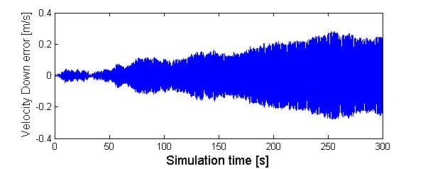
54 Quantity Noise Type Mean Variance Seed GPS Latitude random number 0 1e GPS Longitude random number 0 1e GPS Altitude random number 0 2,5 60 GPS Velocity North random number 0 0, GPS Velocity East random number 0 0, GPS Velocity Down random number 0 0, Table 5.1: GPS noise parametres Sensor Type Mean Size Seed accx random accy random accz random gyrx random 0 4.3e-5 55 gyry random 0 4.3e-5 45 gyrz random 0 4.3e-5 60 Table 5.2: Sensor noise parametres is done mainly by the setting of covariance matrix P initial values. The covariance matrix is a matrix of size 9 9 where the matrix element on the diagonal corresponds to the order of state vector elements. During the tuning of EKF it was observed that the values corresponding to sensor biases influence the performance of the system most significantly. Results from this reduced EKF model are displayed at Figure 5.14 for position and at Figure 5.15 for velocity. Attitude errors are not displayed because noise was not added to gyroscope in this model. When this simplified EKF provided satisfactory results, the system was extended to estimate also corrections to attitude angles and gyroscopes outputs. This step implied the enlargement of state vector, F, G and H matrices and the re-tuning of the entire system. The change of covariance matrix P initial values proved to be insufficient, so the tuning of the system has required also to move Q and R matrix elements. Although a lot of time was spent on EKF tuning, some small issues with stability (mainly in velocity as can be seen in graphs) remained. Nevertheless, the achieved performance of the system is in line with expectations as can be seen at Figure 5.16 (position), 5.17 (velocity) and 5.18 (attitude). 41

55 Figure 5.3: True values of position 42

56 Figure 5.4: True values of velocity 43

57 Figure 5.5: True values of attitude 44

58 Figure 5.6: Position errors from INS with ideal sensors 45

59 Figure 5.7: Velocity errors from INS with ideal sensors 46

60 Figure 5.8: Attitude errors from INS with ideal sensors 47

61 Figure 5.9: Position errors from INS with noisy accelerometers 48

62 Figure 5.10: Velocity errors from INS with noisy accelerometers 49

63 Figure 5.11: Position errors from INS with noisy sensors 50

64 Figure 5.12: Velocity errors from INS with noisy sensors 51

65 Figure 5.13: Attitude errors from noisy sensors 52

66 Figure 5.14: GPS Position errors 53

67 Figure 5.15: GPS Velocity errors 54

68 Figure 5.16: Simple EKF Position errors (noise only in accelerometers) 55

69 Figure 5.17: Simple EKF Velocity errors (noise only in accelerometers) 56

70 Figure 5.18: Full EKF Position errors 57

71 Figure 5.19: Full EKF Velocity errors 58

72 Figure 5.20: Full EKF Attitude errors 59

73 Chapter 6 Conclusion 6.1 Summary The main objective of this thesis is the development of the fully functional algorithm for the inertial navigation system and for the sensor fusion method via Extended Kalman Filter. The parametres of the developed system (choosing INS error model, loosely coupled integration schema etc.) were specified by the assigning company. This thesis presents the necessary knowledge to built the system from INS up to complete solution providing the corrected navigation solution in every step. Chapter 1 presents the brief current status of problematics with references to actual available sources. INS mechanization equations are presented in Chapter 2, including transformation equations and sensor errors outline. Chapter 3 briefly describes Global Positioning System and presents different ways of integration schemas with emphasis on the Extended Kalman filter. One of the most important knowledge is the content of Chapter 4 where the EKF algorithm equations are developed. Chapter 5 displays the achieved results and the last chapter provides the final summary. The major objective was to develop a low-cost INS/GPS navigation system. The research led to following contributions: 1. The discrete form of INS mechanization equations was developed using Laplace and bilinear transformation and succesfully implemented 2. The error analysis of low-cost MEMS sensors was done via Allan Variance to understand sensor behavior 3. The loosely coupled INS/GPS integration algorithm was developed by the use of fifteen-state Extended Kalman Filter 4. The knowledge about designing and tuning EKF was acquired 60

74 6.2 Future work recommendations The further work based on theme of this thesis can involve: dealing with different operational frequencies of fused systems (more information can be found in [17]) comparing different ways to deal with system non-linearity (e.g. Extended Kalman Filter versus Unscented Kalman Filter) research and development in the area of automatic tuning methods (Monte Carlo simulation or similar) more detailed model of sensor errors (algorithm considering bias, scale factor errors and nonorthogonalities is presented e.g. in [3]) more accurate evaluating algorithms (different dynamics of trajectories, simulation of GPS outages, experimental car tests etc.) 6.3 Conclusion The thesis provides the complete solution to implement Extended Kalman Filter for INS and GPS data fusion. During implementation following conclusions were deduced: 1. To ensure correct function of EKF algorithm, proper way to apply corrections back to INS is crucial. The corrections have to be applied inside the loop to apply the corrections before values are delayed and used for next computations. 2. The tuning of EKF is a question of setting proper initial values of covariance matrices P, Q and R. This includes overall 27 values to be set. The major impact has the setting of initial values of covariance matrix P corresponding to biases of sensors (last six numbers). Higher than optimal values cause overestimated bias. Lower values decrease impact of corrections and cause that some noise is not eliminated. 3. The error state EKF algorithm computes corrections at every step. The important fact is that the state vector has to be zeroed at every step. 4. Corrections applied to sensor outputs (computed biases) have to be accumulated 1 in every step to ensure correct processing. 1 Current and previous values are added 61

75 5. Simple EKF model estimating position, velocity and accelerometer errors reduces the following errors achieved after 300 seconds: The error about 3,000 metres in position (altitude) and 20 m/s in velocity (east direction) is reduced to 0.03 metres in position and m/s in velocity. Accuracy of GPS which is used as a measurement fed into EKF is about ten metres in position and 0.03 m/s in velocity. 6. The full EKF model estimating moreover attitude and gyro error has the following results after 300 seconds: The position error is reduced from almost 2,000 metres in latitude to 0.05 metres and the velocity error is reduced from about 25 metres per second in north direction to 0.1 m/s. The attitude error values 0.06 radians have been improved to one third of the noncompensated error. The resulting accuracy in attitude is up to 0.02 radians which corresponds to 1.15 degrees. This accuracy in all parametres is sufficient, but the error behavior in time exhibits a mild instability. This is most probably caused by the tuning which needs more sophisticated methods exceeding the format of master s thesis. 62

76 References 1. Groves, Paul. D.: Principles of GNSS, Inertial and Multisensor Integrated Navigation Systems. Boston, USA: Artech House, p. ISBN-13: Rogers, Robert M.: Applied Mathematics in Integrated Navigation Systems. Third Edition. Reston, USA: American Institute of Aeronautics and Astronautics, p. ISBN-13: Shin, Eun-Hwan: Estimation Techniques for Low-Cost Inertial Navigation. Calgary, Canada: University of Calgary, Department of Geomatics Engineering p. Available from: < 4. Shin, Eun-Hwan: Accuracy Improvement of Low-Cost INS/GPS for Land Application. Calgary, Canada: University of Calgary, Department of Geomatics Engineering, p. Available from: < 5. Farrell, Jay. Barth, Matthew: The Global Positioning System and Inertial Navigation. New York, USA: McGraw-Hill Companies, Inc, p. ISBN X 6. Novák, Jakub: Snímání a zpracování údajů lokalizace dopravního prostředku. Brno: VUT v Brně, Fakulta strojního inzenýrství, p. 7. Horemuž, Milan: Integrated Navigation. Stockholm, Royal Institute of Technology, Division of Geodesy, p. Available from: < %20Integrated%20Navigation.pdf> 8. Gebre-Egziabher, Demoz: GPS, INS and GPS/INS fusion. Minnesota, USA: University of Minnesota, Department of Aerospace Engineering & Mechanics Study material, archiv of autor. 63

77 9. Hrdina, Zdeněk. Pánek, Petr: Rádiové určování polohy (Družicový systém GPS). Praha: ČVUT v Praze, Fakulta elektrotechnická p. ISBN Stockwell, Walter: Bias Stability Measurement : Allan variance. Available from: < 11. Vagner, Martin: MEMS Gyroscope Performance Comparison Using Allan Variance Method. Brno: VUT v Brně, Fakulta elektrotechniky a komunikačních technologií p. Available from: < Doktorske%20projekty/03-Kybernetika%20a%20automatizace/14-xvagne04.pdf> 12. Yang, Yong: Tightly Coupled MEMS INS/GPS Integration with INS Aided Receiver Tracking Loops. Calgary, Canada: University of Calgary, Department of Geomatics Engineering, p. Available from: < 13. Solimeno, Adriano: Low-cost INS/GPS Data Fusion with Extended Kalman Filter for Airborne Applications. Lisabon: Instituto Superior Tecnico p. Available from: < 14. Havlena, Vladimír. Štecha, Jan: Moderní teorie řízení. Praha : ČVUT v Praze, Fakulta elektrotechnická p. ISBN Welch, Greg. Bishop, Gary: An Introduction to the Kalman Filter. Chapel Hill, USA: University of North Carolina, Department of Computer Science p. Available from: < 16. Šimandl, Miroslav: Odhad stavu stochastických systémů. Brno: Centrum pro rozvoj výzkumu pokročilých řídících a senzorických technologií p. Available from: < 17. Farrell, Jay A.: Aided Navigation: GPS with High Rate Sensors. New York, USA: McGraw-Hill Companies, Inc, p. ISBN

78 Appendix A - Content of attached CD Directory Full EKF: FullEKF_2007a.mdl FullEKF_2010a.mdl FullEKF_init.m Directory Simple EKF: SimpleEKF_2007a.mdl SimpleEKF_2010a.mdl SimpleEKF_init.m Directory Trajectories File ReadMe.txt 65

79 Appendix B - Discretization of INS Velocity Update Velocity update equation in the continous form has the following form: v = C n b f b + g n + (2ω n ie + ω n en) v n To avoid the vector product, the skew symmetrix matrix is used: A=(2ω n ie + ω n en) The Laplace transform is applied: sv (s) = C n b f b (s) + g n (s) + AV (s) The Z transform is applied: s = 2 T 1 z z z 1 T 1 + z 1V(z) = Cn b Fb (z) + G(z) AV (z) 2 V (z) (V (z) T 2 ) = Cn b Fb (z) +Cb n F(z) G(z) (z) + G(z) + AV (z) AV T (v k v k 1 ) = C n b Fb k +Cn b Fb k 1 + G k + G k 1 Av k Av k 1 2 T v k + Av k = C n b Fb k +Cn b Fb k 1 + G k + G k T v k 1 Av k 1 66

80 2 T v k(i + A T 2 ) = Cn b Fb k +Cn b Fb k 1 + G k + G k 1 + (I A T 2 )v 2 k 1 T v k = (I + A T [ 2 ) 1 (I A T 2 )v k 1 + T ] 2 (Cn b Fb k +Cn b Fb k 1 + G k + G k 1 ) 67

81 Appendix C - Allan Variance The Allan Variance is a method of measuring frequency stability, mainly of oscillators, clocks or amplifiers. But this method is suitable for simple long term stability analysis at sensors which exhibit non-white noise. The root mean square variation is a sufficient method just for white noise. When this method is applied to non-white noise, the root mean square variation gradually converges to infinity. David W. Allan developed Allan Variance (also known as two-sample variance) to enable convergency in any case. The Allan Variance basic equation can be seen at 6.1. AVAR 2 (τ) = 1 2(n(τ) 1) (y(τ) i+1 y(τ) i ) 2 (6.1) The basic idea is to divide long sequence of data to bins based on an averaging time. Then the difference in average between successive bins are squared, adding them all up and divided by a rescaling factor. The square root of the result is a quantitive measure of how much the average value changed at that particular values of averaging time [10]. Then the procedure is repeated with increased averaging time τ. The result of the procedure is a graph called sigma-tau. The x-axis displays averaging times and the y-axis displays rate in degrees per time interval, usually at log-log scale. The sigmatau graph provides characteristics of several basic noise types according to asymptotics properties. The left side of the graph, short averaging times, the Allan Variance is highest due to noise in sensor. The slope of Allan Variance is a characteristic of angle random walk. As the averaging time increases, the Allan Variance decreases up to the minimum point. From this point Allan Variance starts to increase again due to the rate random walk of the sensor [10]. The minimum point on the curve is the best stability which can be reached with fully modeled sensor and active bias estimation. The rate random walk parametres help predict the time scale at which the drift of sensor occurs [11]. The Allan Variance method was applied to IMU sensors ifog-imu-1-a of imar company. The static tests lasting more than 13 hours were done. The result for accelerometer and gyroscope in x-direction is displayed at Figure 6.1. The bias stability value from Allan Variance gives a better result than the manufacturer indicates. 68

82 Figure 6.1: The Allan Variance on ifog-imu-1-a for accelerometer and gyroscope in x-axis 69